


Multivariate Flagging#
The tutorial aims to introduce the usage of SaQC in the context of some more complex flagging and processing techniques. Mainly we will see how to apply Drift Corrections onto the data and how to perform multivariate flagging.
Data Preparation#
First import the data (from the repository), and generate an saqc instance from it. You will need to download the sensor
data and the
maintenance data
from the repository and make variables datapath and maintpath be
paths pointing at those downloaded files. Note, that the SaQC digests the loaded data in a list.
This is done, to circumvent having to concatenate both datasets in a pandas Dataframe instance, which would introduce
NaN values to both the datasets, wherever their timestamps missmatch. SaQC can handle those unaligned data
internally without introducing artificial fill values to them.
import saqc
import pandas as pd
data = pd.read_csv(datapath, index_col=0)
maint = pd.read_csv(maintpath, index_col=0)
maint.index = pd.DatetimeIndex(maint.index)
data.index = pd.DatetimeIndex(data.index)
qc = saqc.SaQC([data, maint])  # dataframes "data" and "maint" are integrated internally
We can check out the fields, the newly generated SaQC object contains as follows:
>>> qc.data.columns
Index(['sac254_raw', 'level_raw', 'water_temp_raw', 'maint'], dtype='object')
The variables represent meassurements of water level, the specific absorption coefficient at 254 nm Wavelength, the water temperature and there is also a variable, maint, that refers to time periods, where the sac254 sensor was maintained. Lets have a look at those:
>>> qc.data['maint']
Timestamp
2016-01-10 11:15:00    2016-01-10 12:15:00
2016-01-12 14:40:00    2016-01-12 15:30:00
2016-02-10 13:40:00    2016-02-10 14:40:00
2016-02-24 16:40:00    2016-02-24 17:30:00
....                                  ....
2017-10-17 08:55:00    2017-10-17 10:20:00
2017-11-14 15:30:00    2017-11-14 16:20:00
2017-11-27 09:10:00    2017-11-27 10:10:00
2017-12-12 14:10:00    2017-12-12 14:50:00
Name: maint, dtype: object
Measurements collected while maintenance are not trustworthy, so any measurement taken, in any of the listed
intervals should be flagged right away. This can be achieved, with the flagManual() method. Also,
we will flag out-of-range values in the data with the flagRange() method:
>>> qc = qc.flagManual('sac254_raw', mdata='maint', method='closed', label='Maintenance')
>>> qc = qc.flagRange('level_raw', min=0)
>>> qc = qc.flagRange('water_temp_raw', min=-1, max=40)
>>> qc = qc.flagRange('sac254_raw', min=0, max=60)
Lets check out the resulting flags for the sac254 variable with the plot() method:
>>> qc.plot('sac254_raw')
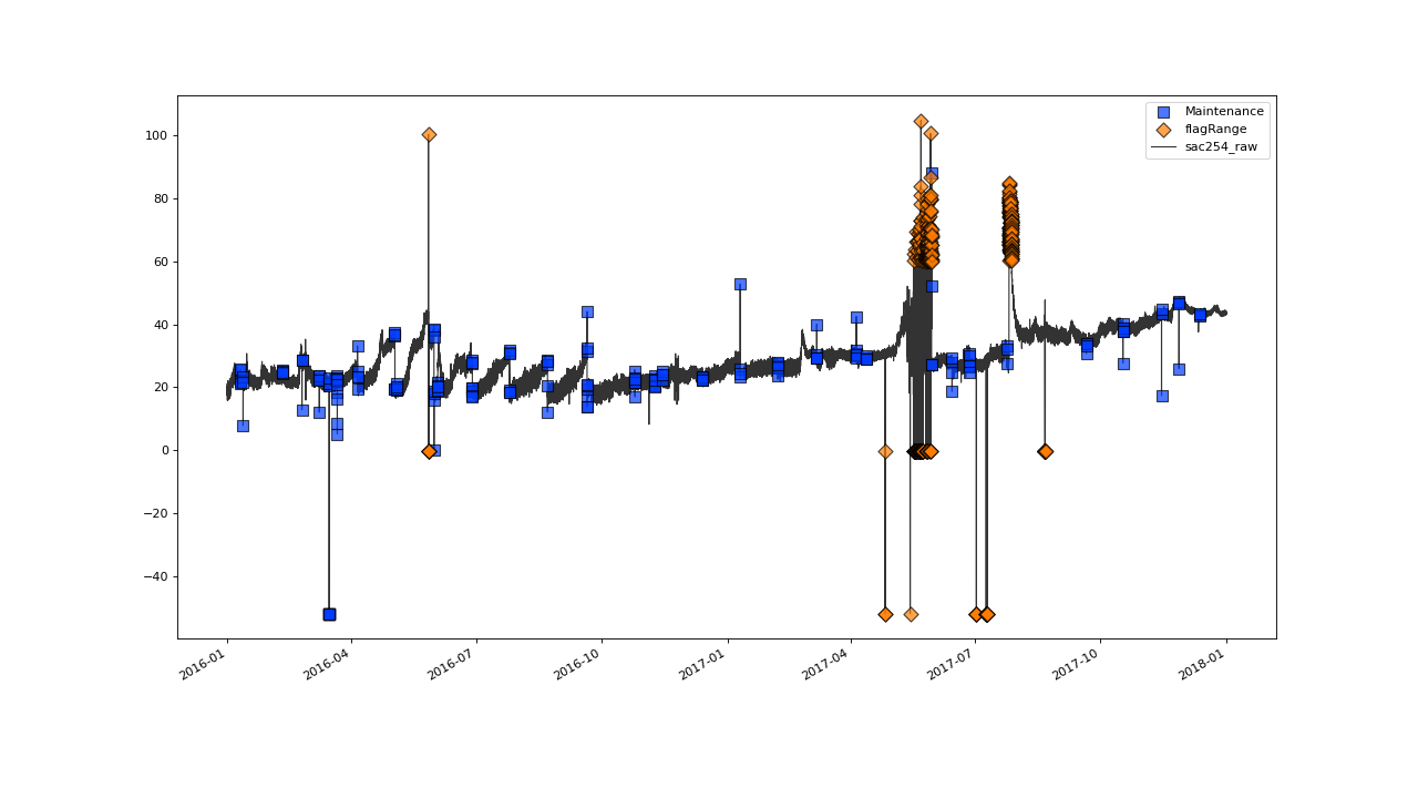
Now we should figure out, what sampling rate the data is intended to have, by accessing the _raw variables
constituting the sensor data. Since saqc.SaQC.data yields a
pandas.DataFrame like object, we can index it with
the desired variables as column names and have a look at the console output to get a first impression.
>>> qc.data[['sac254_raw', 'level_raw', 'water_temp_raw']]
                  sac254_raw |                    level_raw |            water_temp_raw |
============================ | ============================ | ========================= |
2016-01-01 00:02:00  18.4500 | 2016-01-01 00:02:00  103.290 | 2016-01-01 00:02:00  4.84 |
2016-01-01 00:17:00  18.6437 | 2016-01-01 00:17:00  103.285 | 2016-01-01 00:17:00  4.82 |
2016-01-01 00:32:00  18.9887 | 2016-01-01 00:32:00  103.253 | 2016-01-01 00:32:00  4.81 |
2016-01-01 00:47:00  18.8388 | 2016-01-01 00:47:00  103.210 | 2016-01-01 00:47:00  4.80 |
2016-01-01 01:02:00  18.7438 | 2016-01-01 01:02:00  103.167 | 2016-01-01 01:02:00  4.78 |
...                      ... | ...                      ... | ...                   ... |
2017-12-31 22:47:00  43.2275 | 2017-12-31 22:47:00  186.060 | 2017-12-31 22:47:00  5.49 |
2017-12-31 23:02:00  43.6937 | 2017-12-31 23:02:00  186.115 | 2017-12-31 23:02:00  5.49 |
2017-12-31 23:17:00  43.6012 | 2017-12-31 23:17:00  186.137 | 2017-12-31 23:17:00  5.50 |
2017-12-31 23:32:00  43.2237 | 2017-12-31 23:32:00  186.128 | 2017-12-31 23:32:00  5.51 |
2017-12-31 23:47:00  43.7438 | 2017-12-31 23:47:00  186.130 | 2017-12-31 23:47:00  5.53 |
The data seems to have a fairly regular sampling rate of 15 minutes at first glance. But checking out values around 2017-10-29, we notice, that the sampling rate seems not to be totally stable:
>>> qc.data['sac254_raw']['2017-10-29 07:00:00':'2017-10-29 09:00:00']
Timestamp
2017-10-29 07:02:00    40.3050
2017-10-29 07:17:00    39.6287
2017-10-29 07:32:00    39.5800
2017-10-29 07:32:01    39.9750
2017-10-29 07:47:00    39.1350
2017-10-29 07:47:01    40.6937
2017-10-29 08:02:00    40.4938
2017-10-29 08:02:01    39.3337
2017-10-29 08:17:00    41.5238
2017-10-29 08:17:01    38.6963
2017-10-29 08:32:01    39.4337
2017-10-29 08:47:01    40.4987
dtype: float64
Those instabilities do bias most statistical evaluations and it is common practice to apply some alignment onto the data, to obtain a regularly spaced timestamp. (See also the harmonization tutorial for more informations on that topic.)
We will apply linearly obtained alignment to all the sensor data variables,
to interpolate pillar points of multiples of 15 minutes linearly.
>>> qc = qc.align(['sac254_raw', 'level_raw', 'water_temp_raw'], freq='15min')
The resulting timeseries now has has regular timestamp.
>>> qc.data['sac254_raw']
2016-01-01 00:00:00          NaN
2016-01-01 00:15:00    18.617873
2016-01-01 00:30:00    18.942700
2016-01-01 00:45:00    18.858787
2016-01-01 01:00:00    18.756467
                         ...
2017-12-31 23:00:00    43.631540
2017-12-31 23:15:00    43.613533
2017-12-31 23:30:00    43.274033
2017-12-31 23:45:00    43.674453
2018-01-01 00:00:00          NaN
Length: 70177, dtype: float64
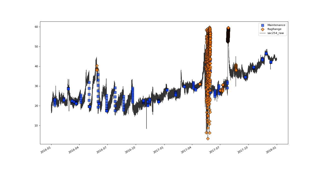
Since points, that were identified as malicous get excluded before the harmonization, the resulting regularly sampled timeseries does not include them anymore:
>>> qc.plot('sac254_raw')
Drift Correction#
The variables SAK254 and Turbidity show drifting behavior originating from dirt, that accumulates on the light
sensitive sensor surfaces over time. The effect, the dirt accumulation has on the measurement values, is assumed to be
properly described by an exponential model. The Sensors are cleaned periodocally, resulting in a periodical reset of
the drifting effect. The Dates and Times of the maintenance events are input to the method
correctDrift(), that will correct the data in between any two such maintenance intervals.
>>> qc = qc.correctDrift('sac254_raw', target='sac254_corrected',maintenance_field='maint', model='exponential')
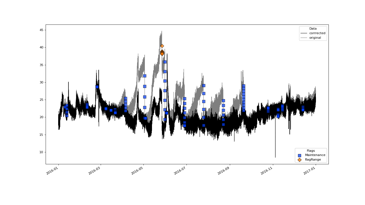
Check out the results for the year 2016
>>> qc.plot(['sac254_raw','sac254_corrected'], xscope='2016', plot_kwargs={'color':['black', 'black'], 'alpha':[.5, 1], 'label':['original', 'corrrected']})
Multivariate Flagging Procedure#
We are basically following the oddWater procedure, as suggested in Talagala, P.D. et al (2019): A Feature-Based Procedure for Detecting Technical Outliers in Water-Quality Data From In Situ Sensors. Water Resources Research, 55(11), 8547-8568.
First, we define a transformation, we want the variables to be transformed with, to make them equally significant in their common feature space. We go for the common pick of just zScoring the variables. Therefor, we just import scipys zscore function and wrap it, so that it will be able to digest nan values, without returning nan.
>>> from scipy.stats import zscore
>>> zscore_func = lambda x: zscore(x, nan_policy='omit')
Now we can pass the function to the transform() method.
>>> qc = qc.transform(['sac254_corrected', 'level_raw', 'water_temp_raw'],
... target=['sac254_norm', 'level_norm', 'water_temp_norm'], func=zscore_func, freq='30D')
The idea of the multivariate flagging approach we are going for, is,
to assign any datapoint a score, derived from the distance this datapoint has to its k nearest
neighbors in feature space. We can do this, via the assignKNNScore() method.
>>> qc = qc.assignKNNScore(field=['sac254_norm', 'level_norm', 'water_temp_norm'],
... target='kNNscores', freq='30D', n=5)
Lets have a look at the resulting score variable.
>>> qc.plot('kNNscores')
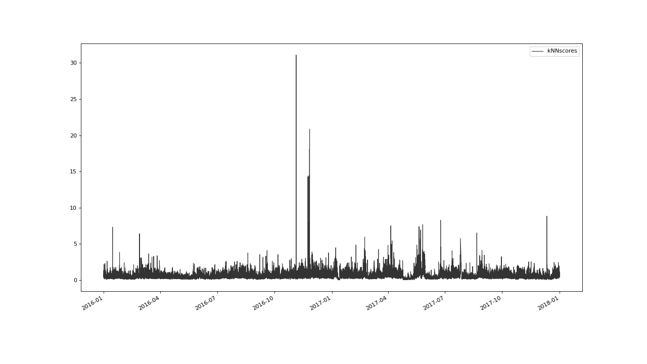
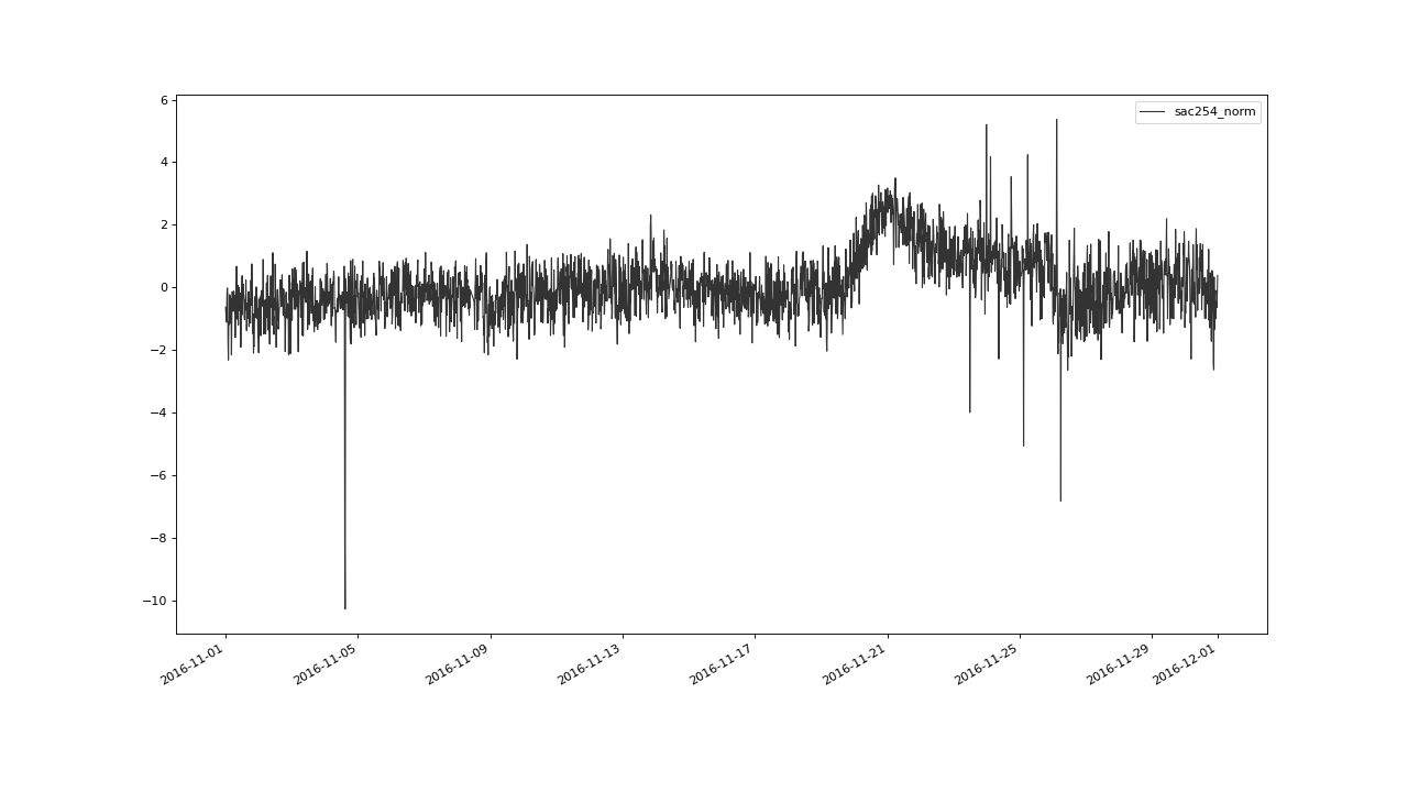
Those scores roughly correlate with the isolation of the scored points in the feature space. For example, have a look at the projection of this feature space onto the 2 dimensional sac - level space, in november 2016:
>>> qc.plot('sac254_norm', phaseplot='level_norm', xscope='2016-11')
We can clearly see some outliers, that seem to be isolated from the cloud of the normalish points. Since those outliers are
correlated with relatively high kNNscores, we could try to calculate a threshold that determines, how extreme an
kNN score has to be to qualify an outlier. Therefor, we will use the saqc-implementation of the
STRAY algorithm, which is available as the method:
flagByStray(). This method will mark some samples of the kNNscore variable as anomaly.
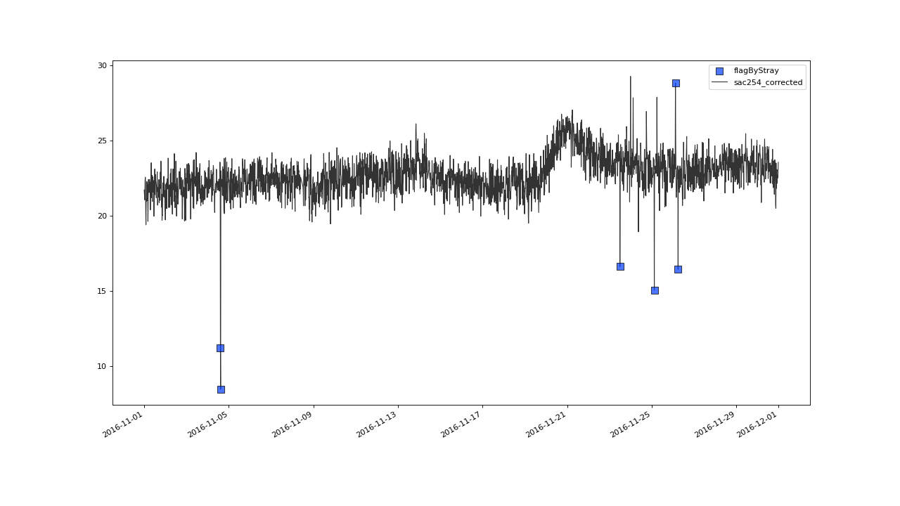
Subsequently we project this marks (or flags) on to the sac variable with a call to
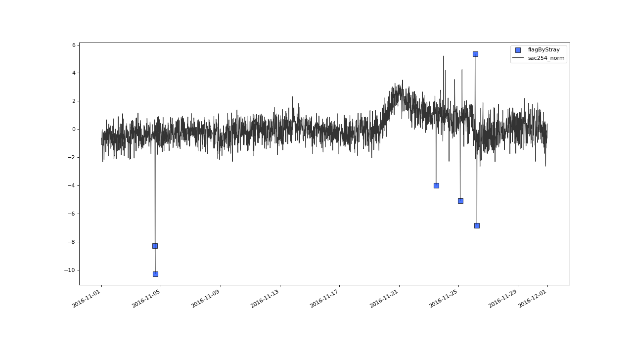
transferFlags(). For the sake of demonstration, we also project the flags
on the normalized sac and plot the flagged values in the sac254_norm - level_norm feature space.
>>> qc = qc.flagByStray(field='kNNscores', freq='30D', alpha=.3)
>>> qc = qc.transferFlags(field='kNNscores', target='sac254_corrected', label='STRAY')
>>> qc = qc.transferFlags(field='kNNscores', target='sac254_norm', label='STRAY')
>>> qc.plot('sac254_corrected', xscope='2016-11')
>>> qc.plot('sac254_norm', phaseplot='level_norm', xscope='2016-11')
Config#
To configure saqc to execute the above data processing and flagging steps, the config file would have to look as follows:
varname                 ; test
#-----------------------;-------------------------------------------
# Data Preparation
sac254_raw              ; flagManual(mdata='maint', method='closed')
level_raw               ; flagRange(min=0)
water_temp_raw          ; flagRange(min=-1)
sac254_raw              ; flagRange(min=0, max=60)
level_raw               ; align(freq='15min')
water_temp_raw          ; align(freq='15min')
sac254_raw              ; align(freq='15min')
# Drift Correcture
sac254_raw              ; correctDrift(target='sac254_corr', maintenance_field='maint', model='exponential')
# Multivariate Flagging Procedure
level_z                 ; transform(field=['level_raw'], func=zScore(x), freq='20D')
water_z                 ; transform(field=['water_temp_raw'], func=zScore(x), freq='20D')
sac_z                   ; transform(field=['sac254_raw'], func=zScore(x), freq='20D')
kNN_scores              ; assignKNNScore(field=['level_z', 'water_z', 'sac_z'], freq='20D')
kNN_scores              ; flagByStray(freq='20D')
level_raw               ; transferFlags(field=['kNN_scores'], label='STRAY')
sac254_corr             ; transferFlags(field=['kNN_scores'], label='STRAY')
water_temp_raw          ; transferFlags(field=['kNN_scores'], label='STRAY')