

Outlier Detection#
The tutorial aims to introduce into a simple to use, jet powerful method for clearing uniformly sampled, univariate
data, from global und local outliers as well as outlier clusters.
Therefor, we will introduce into the usage of the flagUniLOF() method, which represents a
modification of the established Local Outlier Factor (LOF)
algorithm and is applicable without prior modelling of the data to flag.
Example Data Import#
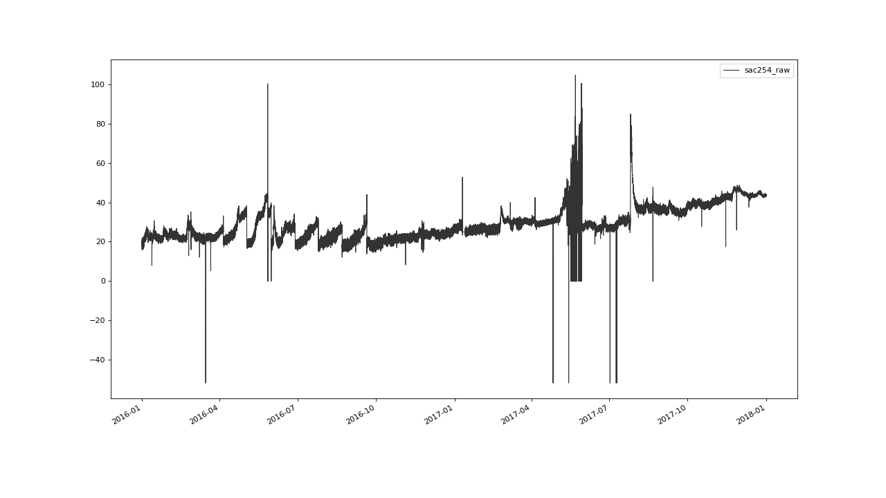
We load the example data set
from the saqc repository using the pandas csv
file reader.
Subsequently, we cast the index of the imported data to DatetimeIndex <https://pandas.pydata.org/docs/reference/api/pandas.DatetimeIndex.html>, then initialize
a SaQC instance using the imported data and finally we plot
it via the built-in plot() method.
>>> import saqc
>>> data = pd.read_csv('./resources/data/hydro_data.csv')
>>> data = data.set_index('Timestamp')
>>> data.index = pd.DatetimeIndex(data.index)
>>> qc = saqc.SaQC(data)
>>> qc.plot('sac254_raw')
Initial Flagging#
We start by applying the algorithm flagUniLOF() with
default arguments, so the main calibration
parameters n and thresh are set to 20 and 1.5
respectively.
For an detailed overview over all the parameters, as well as an introduction
into the working of the algorithm, see the documentation of flagUniLOF()
itself.
>>> import saqc
>>> qc = qc.flagUniLOF('sac254_raw')
>>> qc.plot('sac254_raw')
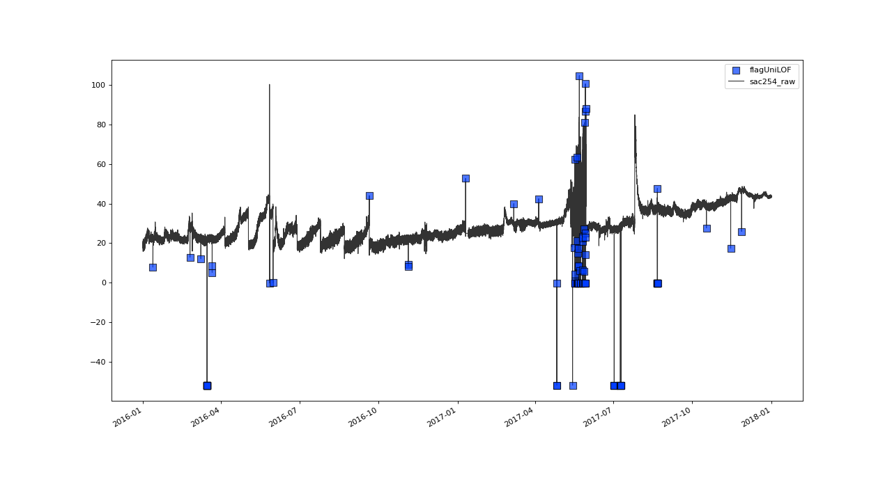
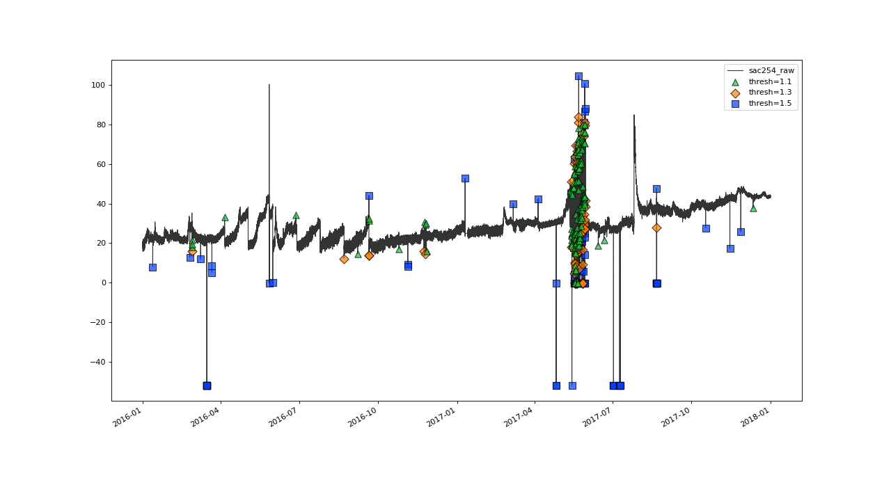
Flagging result with default parameter configuration.#
The results from that initial shot seem to look not too bad.
Most instances of obvious outliers seem to have been flagged right
away and there seem to be no instances of inliers having been falsely labeled.
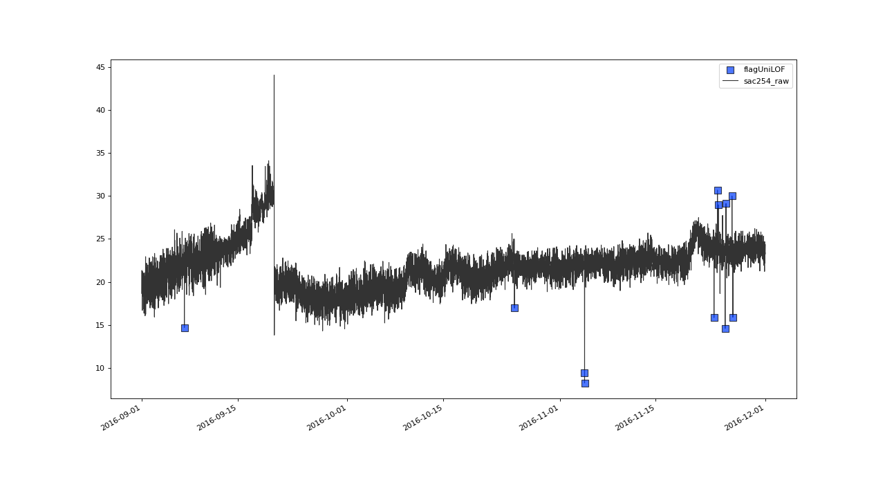
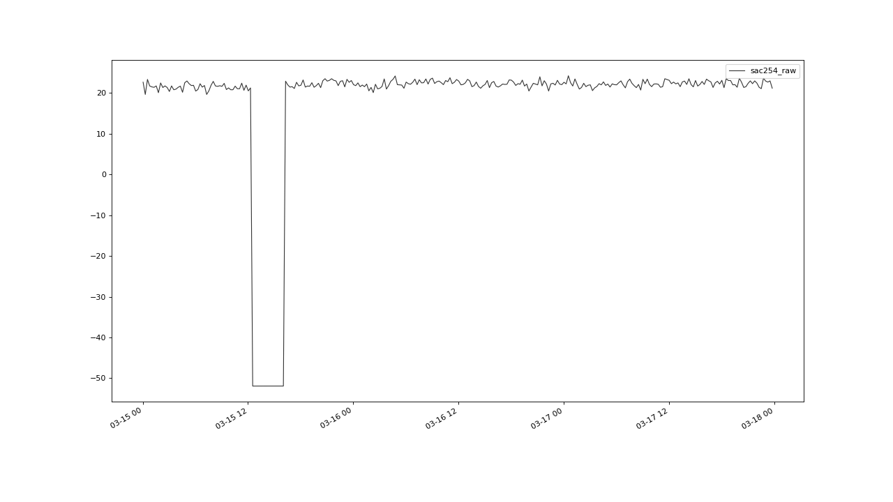
Zooming in onto a 3 months strip on 2016, gives the impression of
some not so extreme outliers having passed flagUniLOF()
undetected:
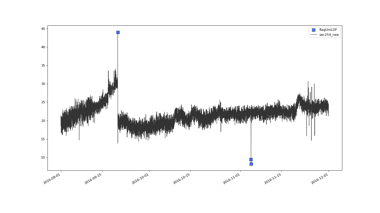
Assuming the flickering values in late september also qualify as outliers, we will see how to tune the algorithm to detect those in the next section.#
Tuning Threshold Parameter#
Of course, the result from applying flagUniLOF() with
default parameter settings might not always meet the expectations.
The best way to tune the algorithm, is, by tweaking one of the
parameters thresh or n.
To tune thresh, find a value that slightly underflags the data,
and reapply the function with evermore decreased values of
thresh.
>>> qc = qc.flagUniLOF('sac254_raw', thresh=1.3, label='threshold = 1.3')
>>> qc.plot('sac254_raw')
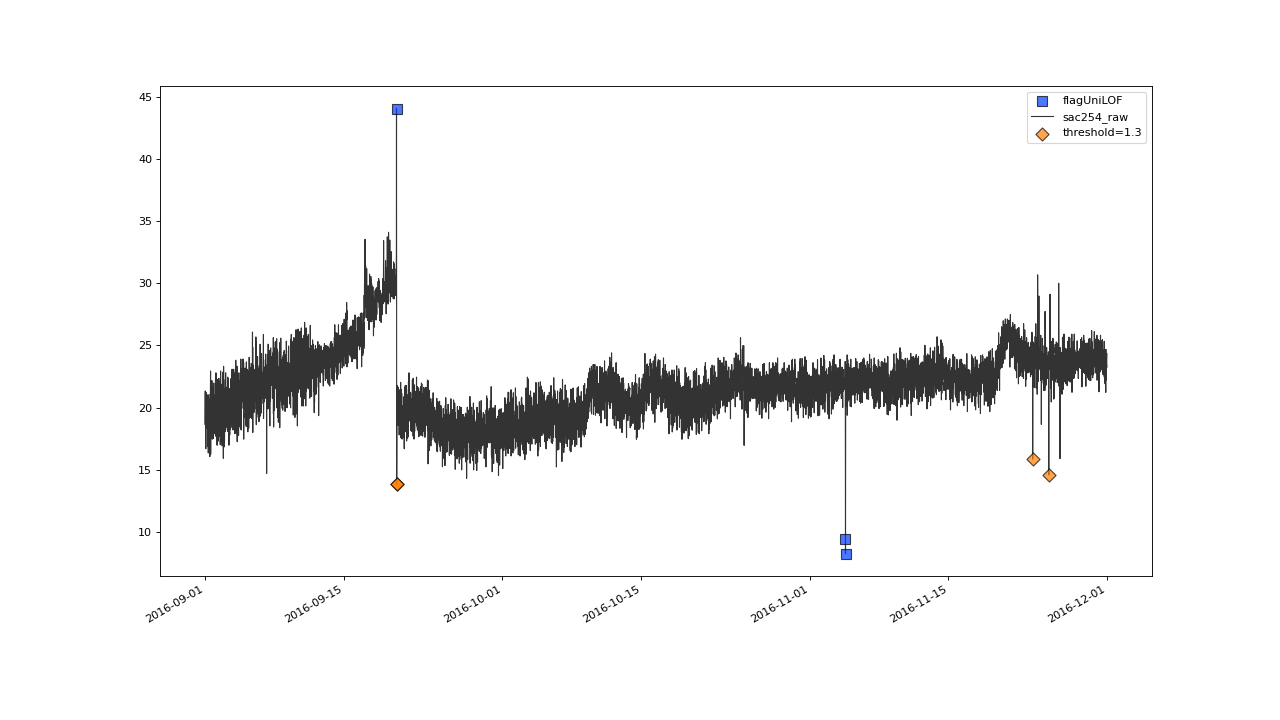
Result from applying flagUniLOF() again on the results for default parameter configuration, this time setting thresh parameter to 1.3.#
It seems we could sift out some more of the outlier like, flickering values. Lets lower the threshold even more:
>>> qc = qc.flagUniLOF('sac254_raw', thresh=1.1, label='threshold = 1.1')
>>> qc.plot('sac254_raw')
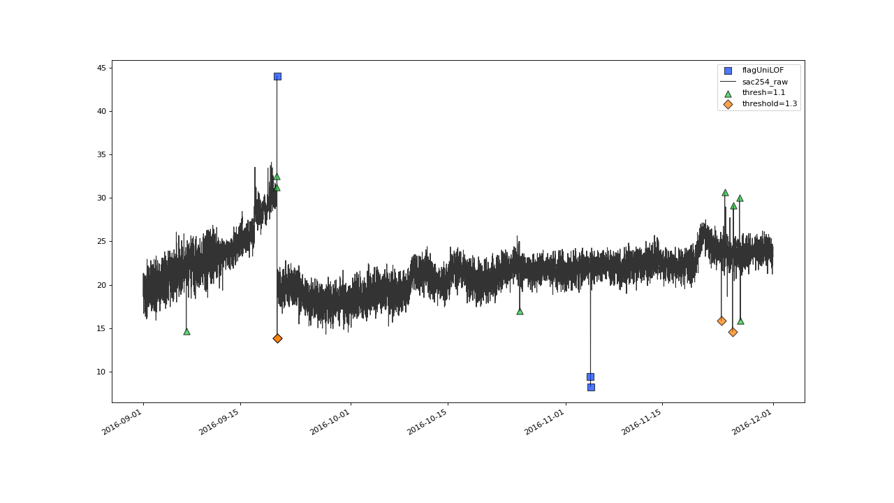
Even more values get flagged with thresh=1.1#
>>> qc = qc.flagUniLOF('sac254_raw', thresh=1.05, label='threshold = 1.05')
>>> qc.plot('sac254_raw')
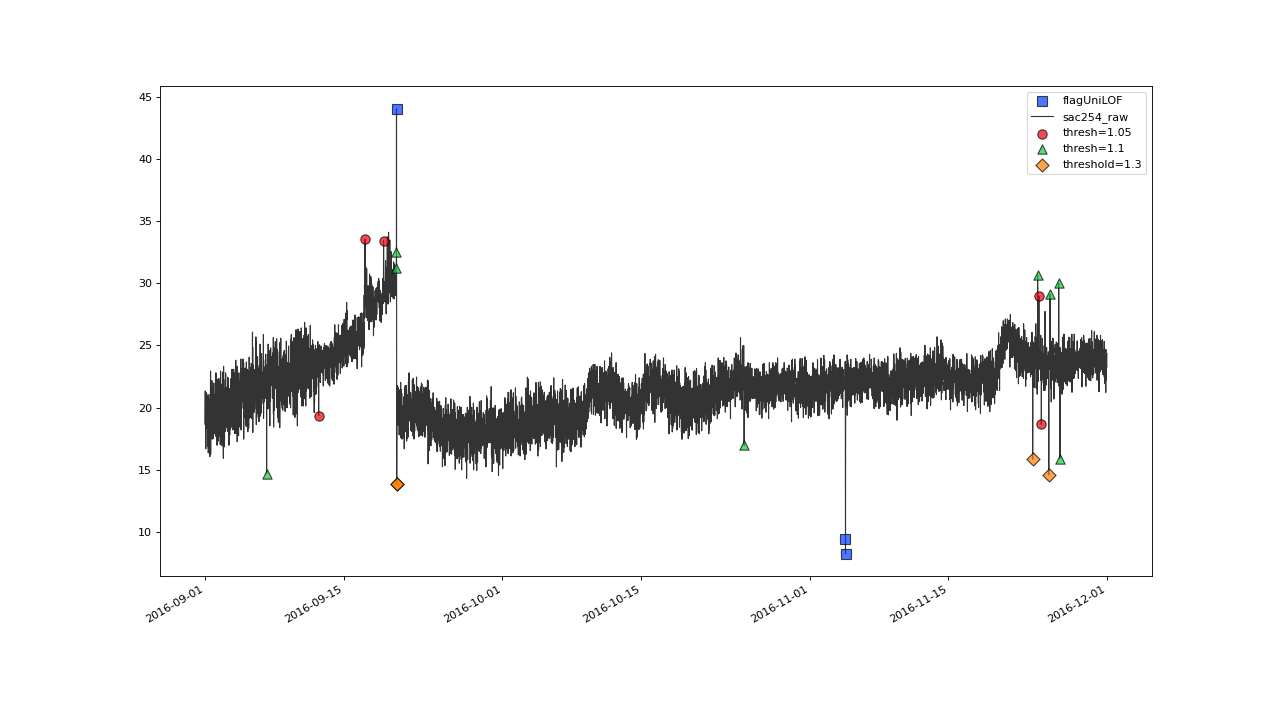
Result begins to look overflagged with thresh=1.05#
The lower bound for meaningful values of thresh is 1.
With threshold 1, the method labels every data point.
>>> qc = qc.flagUniLOF('sac254_raw', thresh=1, label='threshold = 1')
>>> qc.plot('sac254_raw')
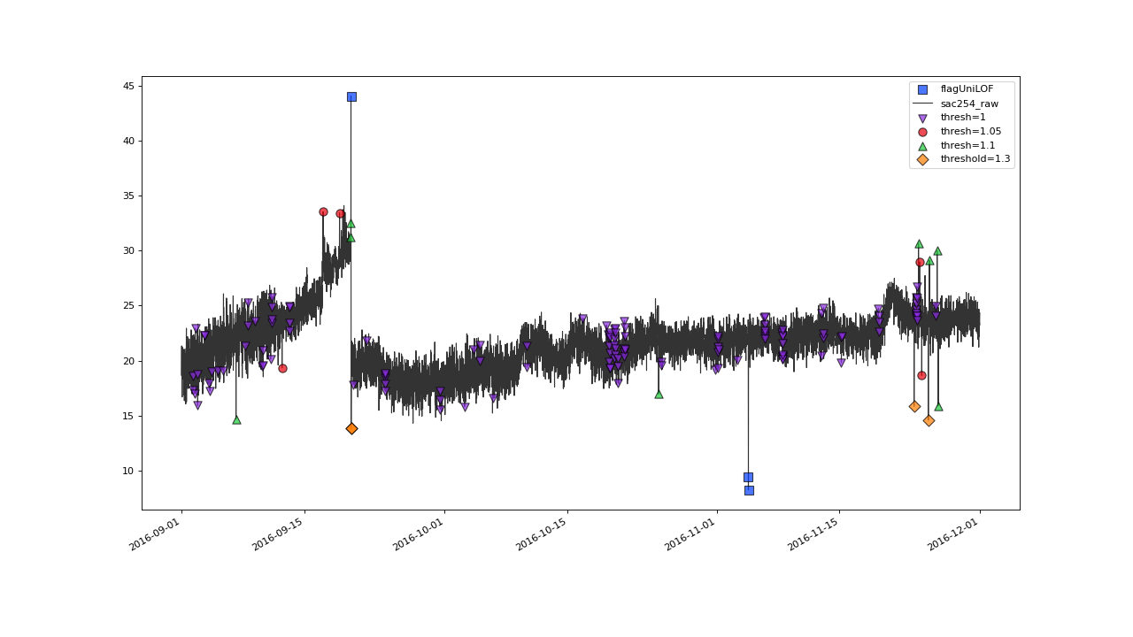
Setting thresh=1 will assign flag to all the values.#
Iterating until 1.1, seems to give quite a good overall flagging result:
Overall the outlier detection with thresh=1.1 seems to work very well. Ideally of course, we would evaluate this result against a validated set of flags while tweaking the parameters.#
The plot shows some over flagging in the closer vicinity of
erratic data jumps.
We will see in the next section, how to fine-tune the algorithm by
shrinking the locality value n to make the process more
robust in the surroundings of anomalies.
Before this, lets briefly check on this outlier cluster, at march 2016, that got correctly flagged, as well.
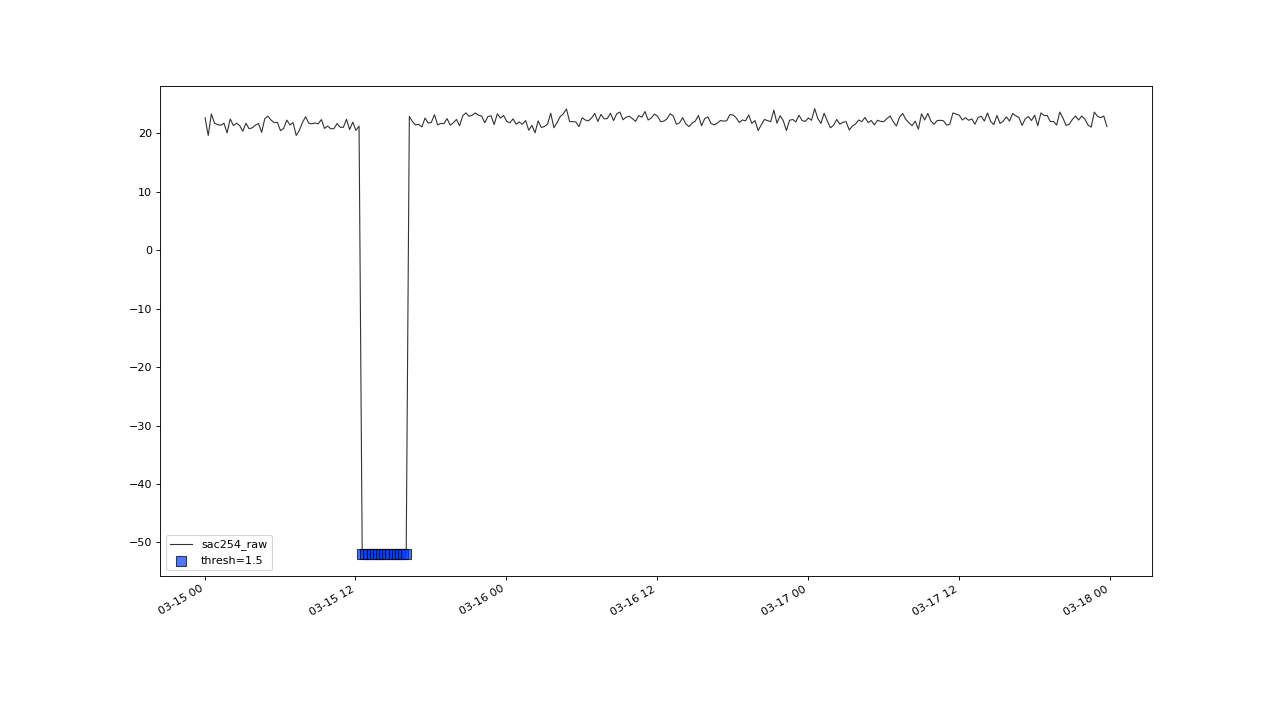
flagUniLOF() will reliably flag groups of outliers, with less than n/2 periods.#
Tuning Locality Parameter#
The parameter n controls the number of nearest neighbors
included into the LOF calculation. So n effectively
determines the size of the “neighborhood”, a data point is compared with, in
order to obtain its “outlierishnes”.
Smaller values of n can lead to clearer results, because of
feedback effects between normal points and outliers getting mitigated:
>>> qc = saqc.SaQC(data)
>>> qc = qc.flagUniLOF('sac254_raw', thresh=1.5, n=8, label='thresh=1.5, n= 8')
>>> qc.plot('sac254_raw', xscope=slice('2016-09','2016-11'))
Result with n=8 and thresh=20#
Since n determines the size of the surrounding,
a point is compared to, it also determines the maximal size of
detectable outlier clusters. The group we were able to detect by applying flagUniLOF()
with n=20, is not flagged with n=8:
A cluster with more than n/2 members, will likely not be detected by the algorithm.#
Also note, that, when changing n, you usually have to restart
calibrating a good starting point for the py:attr:thresh parameter as well.
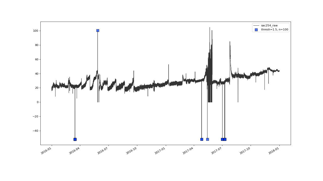
Increasingly higher values of n will
make flagUniLOF() increasingly invariant to local
variance and make it more of a global outlier detection function.
So, an approach towards clearing an entire timeseries from outliers is to start with large n to
clear the data from global outliers first, before fine-tuning thresh for smaller values of n in a second application of the algorithm.
>>> qc = saqc.SaQC(data)
>>> qc = qc.flagUniLOF('sac254_raw', thresh=1.5, n=100, label='thresh=1.5, n=100')
>>> qc.plot('sac254_raw')