

Global Keywords#
Introduction to the usage of the global keywords. (Keywords that can be passed to any saqc.SaQC method.)
Set Up#
Flagging Scheme Constraint#
The Tutorial currently only works when instantiating an SaQC object with the default
flagging scheme, which is the FloatScheme.
Example Data#
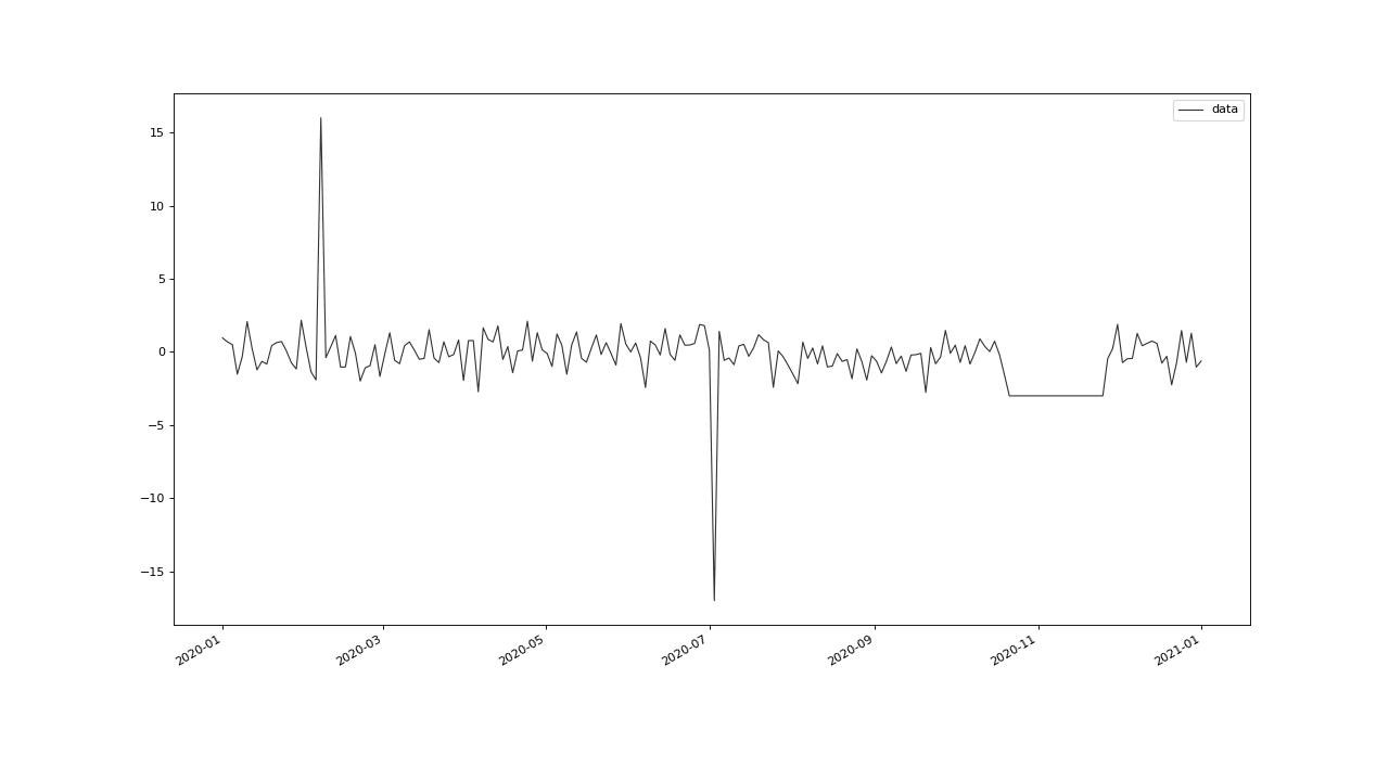
Lets generate some example data and plot it:
>>> import pandas as pd
>>> import numpy as np
>>> noise = np.random.normal(0, 1, 200) # some normally distributed noise
>>> data = pd.Series(noise, index=pd.date_range('2020','2021',periods=200), name='data') # index the noise with some dates
>>> data.iloc[20] = 16 # add some artificial anomalies:
>>> data.iloc[100] = -17
>>> data.iloc[160:180] = -3
>>> qc = saqc.SaQC(data)
>>> qc.plot('data')
Label Keyword#
The label keyword can be passed with any function call and serves as label to be plotted by a subsequent
call to saqc.SaQC.plot().
It is especially useful for enriching figures with custom context information, and for making results from different function calls distinguishable with respect to their purpose and parameterisation. Check out the following example:
At first, we apply some flagging functions to mark anomalies without usage of the label keyword:
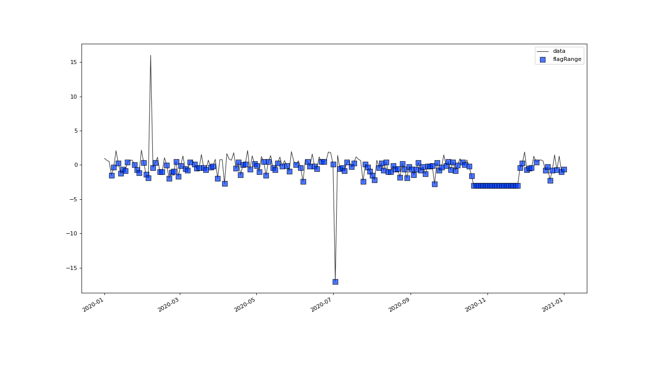
>>> qc = qc.flagRange('data', max=15)
>>> qc = qc.flagRange('data', min=-16)
>>> qc = qc.flagConstants('data', window='2D', thresh=0)
>>> qc = qc.flagManual('data', mdata=pd.Series('2020-05', index=pd.DatetimeIndex(['2020-03'])))
>>> qc.plot('data')
In the above plot, one might want to discern the two results from the call to saqc.SaQC.flagRange() with
respect to the parameters they where called with, also, one might want to give some hints about what is the context of
the flags “manually” determined by the call to saqc.SaQC.flagManual(). Lets repeat the procedure and
enrich the call with this information by making use of the label keyword:
Label Example Usage#
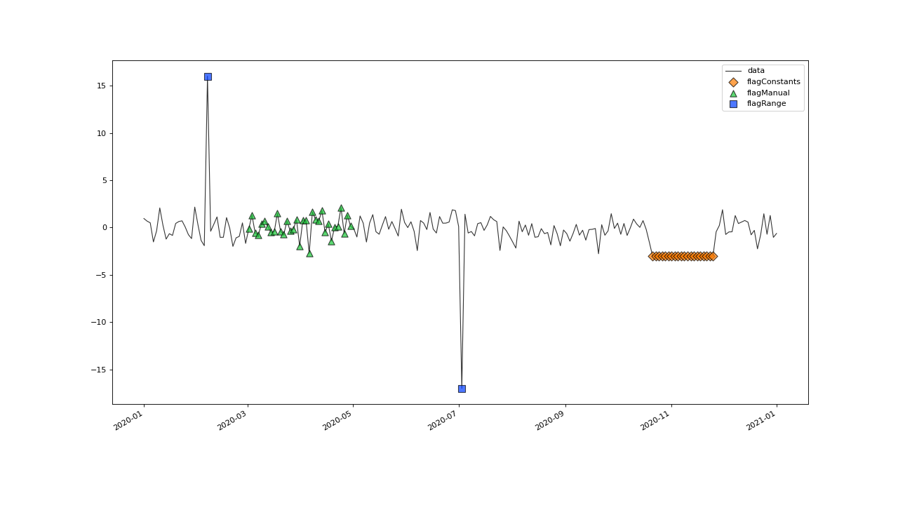
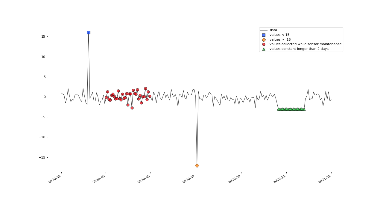
>>> qc = saqc.SaQC(data)
>>> qc = qc.flagRange('data', max=15, label='values < 15')
>>> qc = qc.flagRange('data', min=-16, label='values > -16')
>>> qc = qc.flagConstants('data', window='2D', thresh=0, label='values constant longer than 2 days')
>>> qc = qc.flagManual('data', mdata=pd.Series('2020-05', index=pd.DatetimeIndex(['2020-03'])), label='values collected while sensor maintenance')
>>> qc.plot('data')
dfilter and flag keywords#
The flag keyword controls a tests level of flagging \(f(v)\) for any value \(v\). So,
in short, the keyword controls the output flag level of any flagging function.
The dfilter keyword controls the threshold up to which a flagged value is masked, when passed
on to any flagging function. So, in short, it controls the input threshold, up to which flagged values are visible to
any function that operates on the values.
In more detail: Any value \(v\) with a flag \(f(v)\) will be masked, if \(f(v) >=\) dfilter. A masked value
will appear as NaN (not a number, or missing) to the flagging function and will be numerically treated as such.
(This means, its excluded from most arithmetic calculations, but may be implicitly part of operations, such as count(NaN) or isnan).
Lets at first visualize this interplay with the saqc.SaqC.plot() method. (We are reusing data and code
from the Example Data section). First, we set some flags to the data. As pointed out in
Flagging Scheme Constraint , we are referring to defaultly instantiated saqc.SaQC objects, that use the
FloatScheme , (which uses a real valued scale of flags levels,
ranging from -inf to 255.0).:
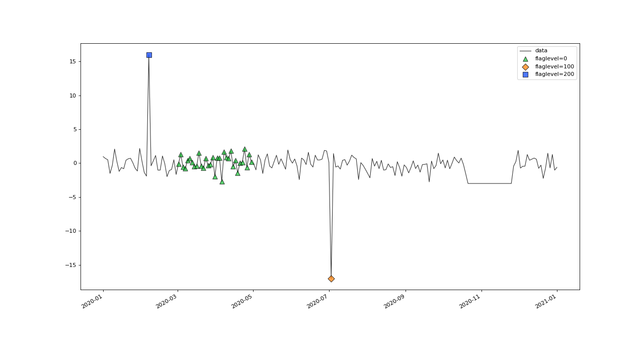
>>> qc = saqc.SaQC(data)
>>> qc = qc.flagRange('data', max=15, label='flaglevel=200', flag=200)
>>> qc = qc.flagRange('data', min=-16, label='flaglevel=100', flag=100)
>>> qc = qc.flagManual('data', mdata=pd.Series('2020-05', index=pd.DatetimeIndex(['2020-03'])), label='flaglevel=0', flag=0)
>>> qc.plot('data')
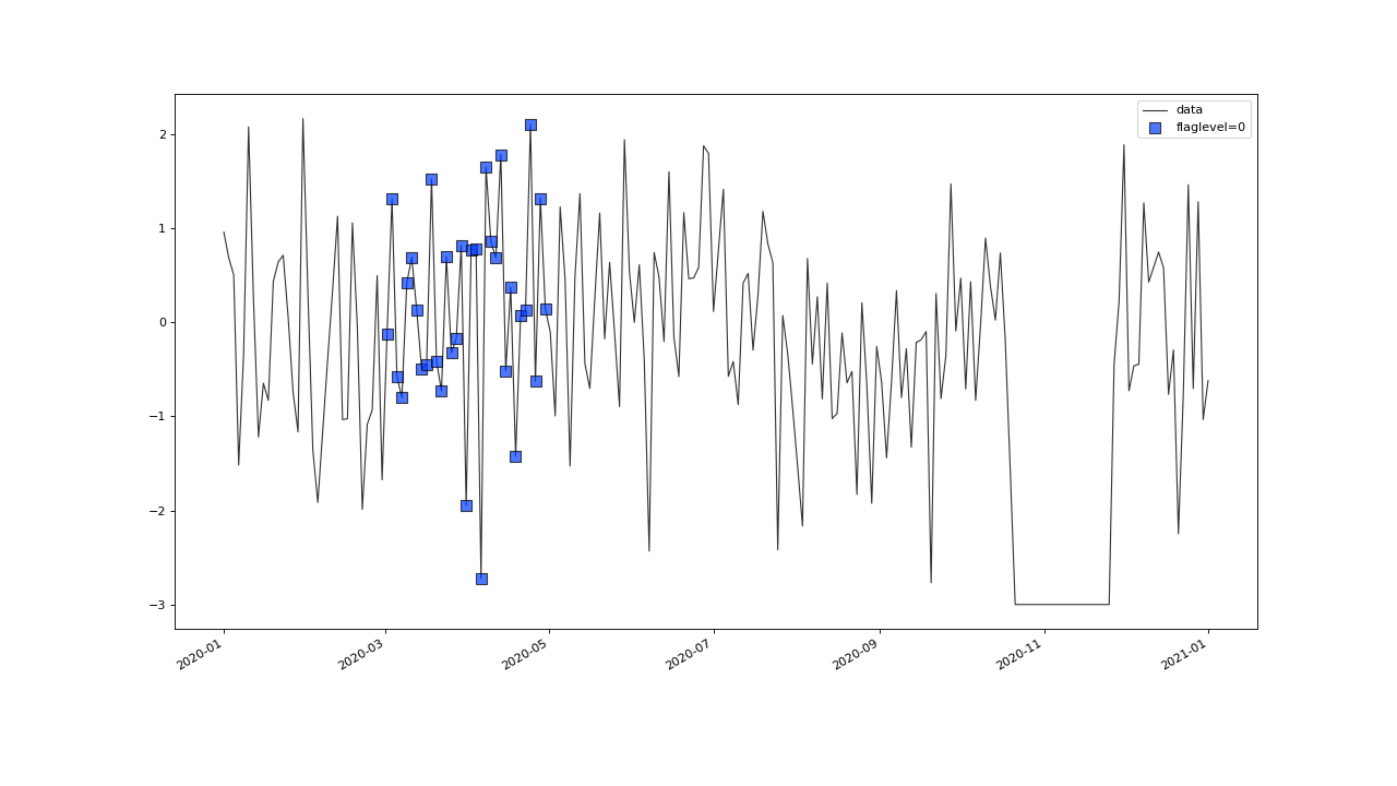
With the dfilter Keyword, we can now control, which of the flags are passed on to the plot function.
For example, if we set dfilter=50, the flags set by the saqc.SaQC.flagRange() method wont get passed on
and thus, the resulting plot will be cleared from the flags:
>>> qc.plot('data', dfilter=50)
Flags of Different Significance#
We can also use the interplay between the dfilter keyword and flag keyword, to order flags priorities.
By default, the dfilter keyword is set to the highest flag value of the instantiated
flagging scheme, referred to, as BAD.
Since the flag set by a test also defaults to BAD, the second call
to saqc.SaQC.flagRange() in the example below, wont get passed the values already flagged by the first call to
saqc.SaQC.flagRange() - so it cant check the value level and assign no additional flag by its self.
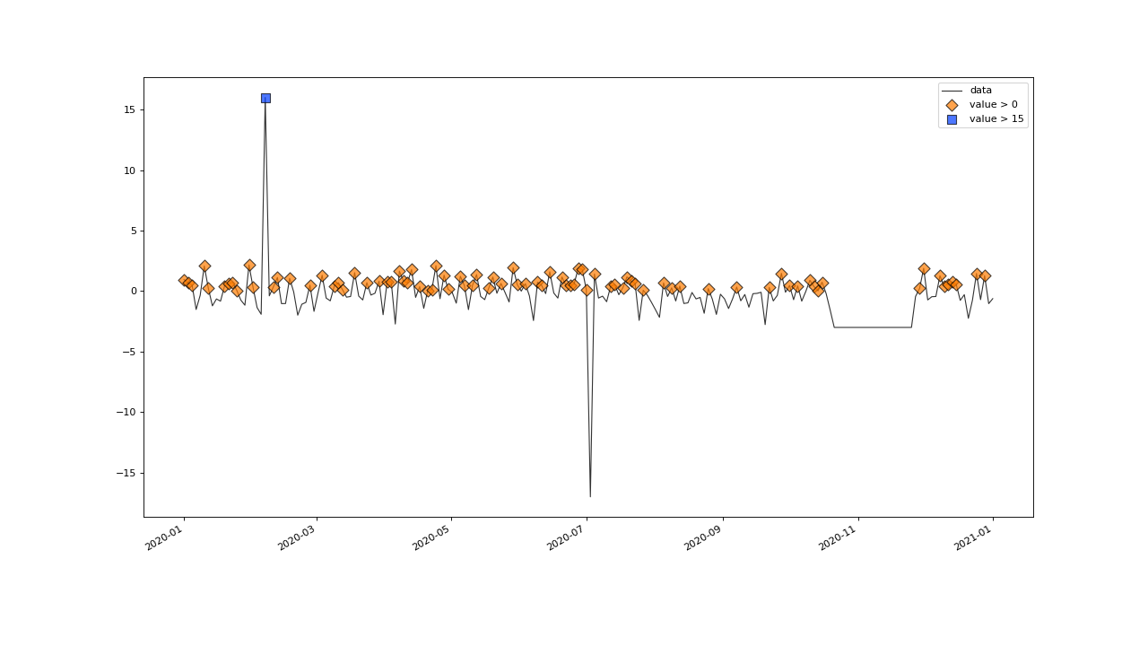
>>> qc = saqc.SaQC(data)
>>> qc = qc.flagRange('data', max=15, label='value > 15')
>>> qc = qc.flagRange('data', max=0, label='value > 0')
>>> qc.plot('data')
We can make the value flagged by both the flagging functions by increasing the
dfilter threshold of the flagging function called second, above the default flag level of
BAD. This can be achieved, by passing the flagging constant
FILTER_NONE,
>>> from saqc.constants import FILTER_NONE
>>> qc = saqc.SaQC(data)
>>> qc = qc.flagRange('data', max=15, label='value > 15')
>>> qc = qc.flagRange('data', max=0, label='value > 0', dfilter=FILTER_NONE)
>>> qc.plot('data')

Unflagging Values#
With the flag keyword it is as also possible, to revoke or unflag a flag from a value.
This way, it is possible to associate flags with conditions determined by other functions.
For example, if we want to flag all values below a level of 0.5, but not those that belong to a constant value
course, we can achieve that, by combining the flag and the dfilter keyword.
Lets first flag all the data below a level of 0.5:
>>> qc = saqc.SaQC(data)
>>> qc = qc.flagRange('data', min=0.5)
>>> qc.plot('data')

Now we can override the flags for the constant value course with the lowest (unflagged) flag level, which, for the
FloatScheme is the value -np.inf. Alternatively to the explicit value, we can use the
UNFLAGGED constant.
Also, for the override to work, we have to rise (or deactivate) the input filter, so that the saqc.SaQC.flagConstants() method
gets the already flagged values passed to test them.
>>> from saqc.constants import UNFLAGGED, FILTER_NONE
>>> qc = qc.flagConstants('data', window='2D', thresh=0, dfilter=FILTER_NONE, flag=UNFLAGGED)
>>> qc.plot('data')