Command Line Application#

Contents#

1. Get toy data and configuration
2. Run SaQC
3. Configure SaQC
- Change test parameters
4. Explore the functionality
- Process multiple variables
- Data harmonization and custom functions

The following passage guides you through the essentials of the usage of SaQC via a toy dataset and a toy configuration.

1. Get toy data and configuration#

If you take a look into the folder saqc/resources/data you will find a toy dataset data.csv which contains the following data:

Date,Battery,SM1,SM2
2016-04-01 00:05:48,3573,32.685,29.3157
2016-04-01 00:20:42,3572,32.7428,29.3157
2016-04-01 00:35:37,3572,32.6186,29.3679
2016-04-01 00:50:32,3572,32.736999999999995,29.3679
2016-04-01 01:05:26,3572,32.736999999999995,29.3131

These are the first entries of two timeseries of soil moisture (SM1+2) and the battery voltage of the measuring device over time. Generally, this is the way that your data should look like to run saqc. Note, however, that you do not necessarily need a series of dates to reference to and that you are free to use more columns of any name that you like.

Now have a look at a basic sonfiguration file, as this one. It contains the following lines:

varname;test
#------;--------------------------
SM2    ;flagRange(min=10, max=60)
SM2    ;flagZScore(window="30d", thresh=3.5, method="modified", center=False)
SM2    ;plot()

These lines illustrate how different quality control tests can be specified for different variables, for a more detailed explanation of the configuration format, please refer to respective documentation page

In this case, we trigger a range test, that flags all values exceeding the range of the bounds of the interval [10,60]. Subsequently, a test to detect spikes, is applied, using the MAD-method. (flagMAD()). You can find an overview of all available quality control tests here. Note that the tests are executed in the order that you define in the configuration file. The quality flags that are set during one test are always passed on to the subsequent one.

2. Run SaQC#

On Unix/Mac-systems#

Remember to have your virtual environment activated:

source env_saqc/bin/activate

From here, you can run saqc and tell it to run the tests from the toy config-file on the toy dataset via the -c and -d options:

python3 -m saqc -c docs/resources/data/myconfig.csv -d docs/resources/data/data.csv

On Windows#

cd env_saqc/Scripts
./activate

Via your console, move into the folder you downloaded saqc into:

cd saqc

From here, you can run saqc and tell it to run the tests from the toy config-file on the toy dataset via the -c and -d options:

py -3 -m saqc -c docs/resources/data/myconfig.csv -d docs/resources/data/data.csv

If you installed saqc via PYPi, you can omit sh python -m.

The command will output this plot:

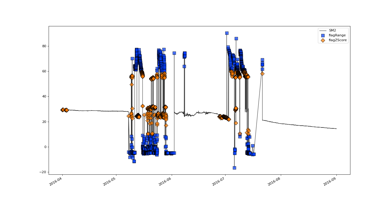
So, what do we see here?

The plot shows the data as well as the quality flags that were set by the tests for the variable SM2, as defined in the config-file
Following our definition in the config-file, first the flagRange() -test that flags all values outside the range [10,60] was executed and after that, the flagMAD() -test to identify spikes in the data
Finally we triggered the generation of a plot, by adding the plot() function in the last line.

Save outputs to file#

If you want the final results to be saved to a csv-file, you can do so by the use of the -o option:

saqc -c docs/resources/data/config.csv -d docs/resources/data/data.csv -o out.csv

Which saves a dataframe that contains both the original data and the quality flags that were assigned by SaQC for each of the variables:

Date,SM1,SM1_flags,SM2,SM2_flags
2016-04-01 00:05:48,32.685,OK,29.3157,OK
2016-04-01 00:20:42,32.7428,OK,29.3157,OK
2016-04-01 00:35:37,32.6186,OK,29.3679,OK
2016-04-01 00:50:32,32.736999999999995,OK,29.3679,OK
...

3. Configure SaQC#

Change test parameters#

Now you can start to change the settings in the config-file and investigate the effect that has on how many datapoints are flagged as “BAD”. When using your own data, this is your way to configure the tests according to your needs. For example, you could modify your myconfig.csv and change the parameters of the range-test:

varname;test
#------;--------------------------
SM2    ;flagRange(min=-20, max=60)
SM2    ;flagZScore(window="30d", thresh=3.5, method='modified', center=False)
SM2    ;plot()

Rerunning SaQC as above produces the following plot:

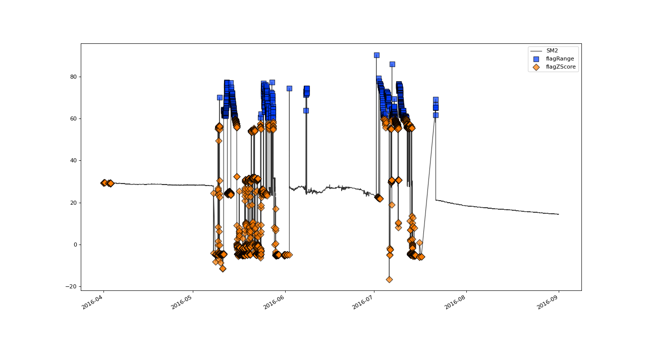
You can see that the changes that we made to the parameters of the range test take effect so that only the values > 60 are flagged by it (black points). This, in turn, leaves more erroneous data that is then identified by the proceeding spike-test (red points).

4. Explore the functionality#

Process multiple variables#

You can also define multiple tests for multiple variables in your data. These are then executed sequentially and can be plotted seperately. To not interrupt processing, the plots get stored to files. (We route the storage to the repos resources folder…)

varname;test
#------;--------------------------
SM1;flagRange(min=10, max=60)
SM2;flagRange(min=10, max=60)
SM1;flagZScore(window="15d", thresh=3.5, method='modified')
SM2;flagZScore(window="30d", thresh=3.5, method='modified')
SM1;plot(path='../resources/temp/SM1processingResults')
SM2;plot(path='../resources/temp/SM2processingResults')

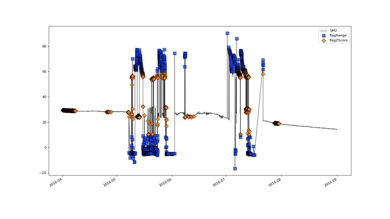
which gives you separate plots for each call to plot:

SM1	SM2

Data harmonization and custom functions#

SaQC includes functionality to harmonize the timestamps of one or more data series. Also, you can write your own tests using a python-based extension language. This would look like this:

varname;test
#------;--------------------------
SM2    ;align(freq="15Min",method="nshift")
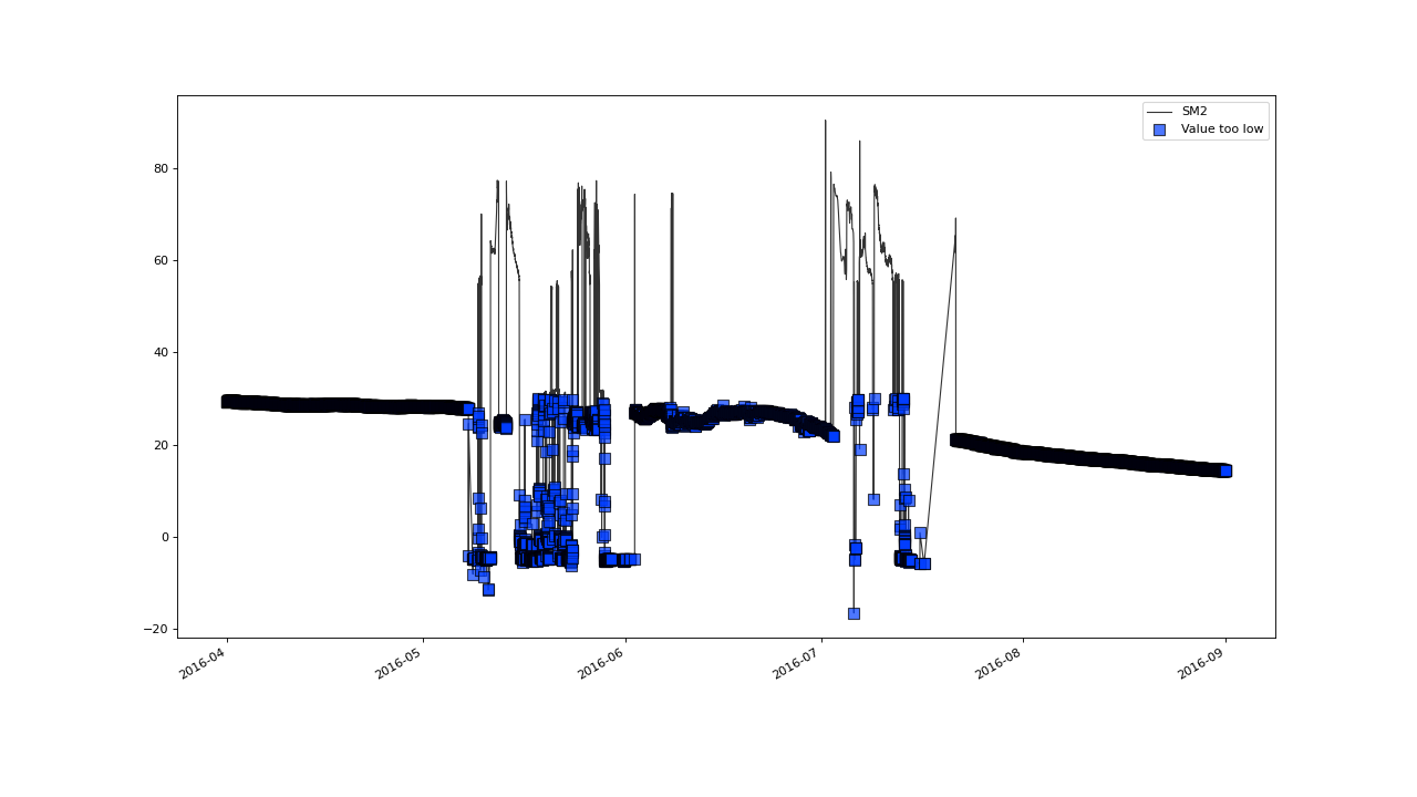
SM2    ;flagGeneric(func=(SM2 < 30), label='Value too low')
SM2    ;plot()

The above executes an internal framework that aligns the timestamps of SM2 to a 15min-grid (saqc.SaQC.shift()). Further information on harmonization can be found in the Resampling cookbook.

,Battery,SM1,SM2
2016-04-01 00:00:00,,,29.3157
2016-04-01 00:05:48,3573.0,32.685,
2016-04-01 00:15:00,,,29.3157
2016-04-01 00:20:42,3572.0,32.7428,
2016-04-01 00:30:00,,,29.3679
2016-04-01 00:35:37,3572.0,32.6186,
2016-04-01 00:45:00,,,29.3679
2016-04-01 00:50:32,3572.0,32.736999999999995,
2016-04-01 01:00:00,,,29.3131

Also, all values where SM2 is below 30 are flagged via the custom function (see plot below) and the plot is labeled with the string passed to the label keyword. You can learn more about the syntax of these custom functions here.