SaQC#

class SaQC(data=None, flags=None, scheme='float')[source]#

Bases: FunctionsMixin

Attributes Summary

`attrs`	Dictionary of global attributes of this dataset.
`columns`
`data`
`flags`
`scheme`

Methods Summary

`align`(field, freq[, method, order, overwrite])	Convert time series to specified frequency.
`andGroup`(field[, group, target, flag])	Logical AND operation for Flags.
`assignChangePointCluster`(field, stat_func, ...)	Label data where it changes significantly.
`assignKNNScore`(field, target[, n, func, ...])	Score datapoints by an aggregation of the distances to their k nearest neighbors.
`assignLOF`(field, target[, n, freq, ...])	Assign Local Outlier Factor (LOF).
`assignRegimeAnomaly`(field, cluster_field, spread)	A function to detect values belonging to an anomalous regime regarding modelling regimes of field.
`assignUniLOF`(field[, n, algorithm, p, ...])	Assign "univariate" Local Outlier Factor (LOF).
`assignZScore`(field[, window, norm_func, ...])	Calculate (rolling) Zscores.
`calculatePolynomialResiduals`(field, window, ...)	Fits a polynomial model to the data and calculate the residuals.
`calculateRollingResiduals`(field, window[, ...])	Calculate the diff of a rolling-window function and the data.
`clearFlags`(field, **kwargs)	Assign UNFLAGGED value to all periods in field.
`concatFlags`(field[, target, method, invert, ...])	Project flags/history of `field` to `target` and adjust to the frequeny grid of `target` by 'undoing' former interpolation, shifting or resampling operations
`copy`([deep])
`copyField`(field, target[, overwrite])	Make a copy of the data and flags of field.
`correctDrift`(field, maintenance_field, model)	The function corrects drifting behavior.
`correctOffset`(field, max_jump, spread, ...)	type field: `str`
`correctRegimeAnomaly`(field, cluster_field, model)	Function fits the passed model to the different regimes in data[field] and tries to correct those values, that have assigned a negative label by data[cluster_field].
`dropField`(field, **kwargs)	Drops field from the data and flags.
`fitLowpassFilter`(field, cutoff[, nyq, ...])	Fits the data using the butterworth filter.
`fitPolynomial`(field, window, order[, ...])	Fits a polynomial model to the data.
`flagByClick`(field[, max_gap, gui_mode, ...])	Pop up GUI for adding or removing flags by selection of points in the data plot.
`flagByGrubbs`(field, window[, alpha, ...])	Flag outliers using the Grubbs algorithm.
`flagByScatterLowpass`(field, window, thresh)	Flag data chunks of length `window` dependent on the data deviation.
`flagByStatLowPass`(field, window, thresh[, ...])	Flag data chunks of length `window` dependent on the data deviation.
`flagByStray`(field[, window, min_periods, ...])	Flag outliers in 1-dimensional (score) data using the STRAY Algorithm.
`flagByVariance`(field, window, thresh[, ...])	Flag low-variance data.
`flagChangePoints`(field, stat_func, ...[, ...])	Flag values that represent a system state transition.
`flagConstants`(field, thresh, window[, ...])	Flag constant data values.
`flagDriftFromNorm`(field, window, spread[, ...])	Flags data that deviates from an avarage data course.
`flagDriftFromReference`(field, reference, ...)	Flags data that deviates from a reference course.
`flagDummy`(field, **kwargs)	Function does nothing but returning data and flags.
`flagGeneric`(field, func[, target, flag])	Flag data based on a given function.
`flagIsolated`(field, gap_window, group_window)	Find and flag temporal isolated groups of data.
`flagJumps`(field, thresh, window[, ...])	Flag jumps and drops in data.
`flagLOF`(field[, n, thresh, algorithm, p, flag])	Flag values where the Local Outlier Factor (LOF) exceeds cutoff.
`flagMAD`(field[, window, z, min_residuals, ...])	Flag outiers using the modified Z-score outlier detection method.
`flagMVScores`(field[, trafo, alpha, n, func, ...])	The algorithm implements a 3-step outlier detection procedure for simultaneously flagging of higher dimensional data (dimensions > 3).
`flagManual`(field, mdata[, method, mformat, ...])	Include flags listed in external data.
`flagMissing`(field[, flag, dfilter])	Flag NaNs in data.
`flagOffset`(field, tolerance, window[, ...])	A basic outlier test that works on regularly and irregularly sampled data.
`flagPatternByDTW`(field, reference[, ...])	Pattern Recognition via Dynamic Time Warping.
`flagRaise`(field, thresh, raise_window, freq)	The function flags raises and drops in value courses, that exceed a certain threshold within a certain timespan.
`flagRange`(field[, min, max, flag])	Function flags values exceeding the closed interval [`min`, `max`].
`flagRegimeAnomaly`(field, cluster_field, spread)	Flags anomalous regimes regarding to modelling regimes of `field`.
`flagUnflagged`(field[, flag])	Function sets a flag at all unflagged positions.
`flagUniLOF`(field[, n, thresh, algorithm, p, ...])	Flag "univariate" Local Outlier Factor (LOF) exceeding cutoff.
`flagZScore`(field[, method, window, thresh, ...])	Flag data where its (rolling) Zscore exceeds a threshold.
`forceFlags`(field[, flag])	Set whole column to a flag value.
`interpolateByRolling`(field, window[, func, ...])	Replace NaN by the aggregation result of the surrounding window.
`orGroup`(field[, group, target, flag])	Logical OR operation for Flags.
`plot`(field[, path, max_gap, mode, history, ...])	Plot data and flags or store plot to file.
`processGeneric`(field, func[, target, dfilter])	Generate/process data with user defined functions.
`propagateFlags`(field, window[, method, ...])	Flag values before or after flags set by the last test.
`reindex`(field, index[, method, tolerance, ...])	Change a variables index.
`renameField`(field, new_name, **kwargs)	Rename field in data and flags.
`resample`(field, freq[, func, method, maxna, ...])	Resample data points and flags to a regular frequency.
`rolling`(field, window[, target, func, ...])	Calculate a rolling-window function on the data.
`selectTime`(field, mode[, selection_field, ...])	Realizes masking within saqc.
`setFlags`(field, data[, override, flag])	Include flags listed in external data.
`transferFlags`(field[, target, squeeze, ...])	Transfer Flags of one variable to another.
`transform`(field, func[, freq])	Transform data by applying a custom function on data chunks of variable size.

Attributes Documentation

attrs#: Dictionary of global attributes of this dataset.

columns#

data#

flags#

scheme#

Methods Documentation

align(field, freq, method='time', order=2, overwrite=False, **kwargs)#

Convert time series to specified frequency. Values affected by frequency changes will be inteprolated using the given method.

Parameters:

field (str | list[str]) – Variable to process.
freq (str) – Target frequency.
method (str (default: 'time')) –
Interpolation technique to use. One of:
- 'nshift': Shift grid points to the nearest time stamp in the range = +/- 0.5 * freq.
- 'bshift': Shift grid points to the first succeeding time stamp (if any).
- 'fshift': Shift grid points to the last preceeding time stamp (if any).
- 'linear': Ignore the index and treat the values as equally spaced.
- 'time', 'index', 'values': Use the actual numerical values of the index.
- 'pad': Fill in NaNs using existing values.
- 'spline', 'polynomial': Passed to scipy.interpolate.interp1d. These methods use the numerical values of the index. An order must be specified, e.g. qc.interpolate(method='polynomial', order=5).
- 'nearest', 'zero', 'slinear', 'quadratic', 'cubic', 'barycentric': Passed to scipy.interpolate.interp1d. These methods use the numerical values of the index.
- 'krogh', 'spline', 'pchip', 'akima', 'cubicspline': Wrappers around the SciPy interpolation methods of similar names.
- 'from_derivatives': Refers to scipy.interpolate.BPoly.from_derivatives.
order (int (default: 2)) – Order of the interpolation method, ignored if not supported by the chosen method.
extrapolate –
Use parameter to perform extrapolation instead of interpolation onto the trailing and/or leading chunks of NaN values in data series.
- None (default) - perform interpolation
- 'forward'/'backward' - perform forward/backward extrapolation
- 'both' - perform forward and backward extrapolation
overwrite (bool (default: False)) – If set to True, existing flags will be cleared.
target (str | list[str], optional) – Variable name to which the results are written. target will be created if it does not exist. Defaults to field.
dfilter (Any, optional) – Defines which observations will be masked based on the already existing flags. Any data point with a flag equal or worse to this threshold will be passed as NaN to the function. Defaults to the DFILTER_ALL value of the translation scheme.
flag (Any, optional) – The flag value the function uses to mark observations. Defaults to the BAD value of the translation scheme.

Returns:

SaQC – the updated SaQC object

Return type:

saqc.SaQC

andGroup(field, group=None, target=None, flag=255.0, **kwargs)#

Logical AND operation for Flags.

Flag the variable(s) field at every period, at wich field in all of the saqc objects in group is flagged.

See Examples section for examples.

Parameters:

field (str | list[str]) – Variable to process.
group (Optional[Sequence[SaQC]] (default: None)) – A collection of SaQC objects. Flag checks are performed on all SaQC objects based on the variables specified in field. Whenever all monitored variables are flagged, the associated timestamps will receive a flag.
target (str | list[str], optional) – Variable name to which the results are written. target will be created if it does not exist. Defaults to field.
dfilter (Any, optional) – Defines which observations will be masked based on the already existing flags. Any data point with a flag equal or worse to this threshold will be passed as NaN to the function. Defaults to the DFILTER_ALL value of the translation scheme.
flag (Any, optional) – The flag value the function uses to mark observations. Defaults to the BAD value of the translation scheme.

Returns:

SaQC – the updated SaQC object

Return type:

saqc.SaQC

Examples

Flag data, if the values are above a certain threshold (determined by flagRange()) AND if the values are constant for 3 periods (determined by flagConstants())

>>> dat = pd.Series([1,0,0,0,1,2,3,4,5,5,5,4], name='data', index=pd.date_range('2000', freq='10min', periods=12))
>>> qc = saqc.SaQC(dat)
>>> qc = qc.andGroup('data', group=[qc.flagRange('data', max=4), qc.flagConstants('data', thresh=0, window=3)])
>>> qc.flags['data']
2000-01-01 00:00:00     -inf
2000-01-01 00:10:00     -inf
2000-01-01 00:20:00     -inf
2000-01-01 00:30:00     -inf
2000-01-01 00:40:00     -inf
2000-01-01 00:50:00     -inf
2000-01-01 01:00:00     -inf
2000-01-01 01:10:00     -inf
2000-01-01 01:20:00    255.0
2000-01-01 01:30:00    255.0
2000-01-01 01:40:00    255.0
2000-01-01 01:50:00     -inf
Freq: 10min, dtype: float64

Masking data, so that a test result only gets assigned during daytime (between 6 and 18 o clock for example). The daytime condition is generated via flagGeneric():

>>> from saqc.lib.tools import periodicMask
    >>> mask_func = lambda x: ~periodicMask(x.index, '06:00:00', '18:00:00', True)
>>> dat = pd.Series(range(100), name='data', index=pd.date_range('2000', freq='4h', periods=100))
>>> qc = saqc.SaQC(dat)
>>> qc = qc.andGroup('data', group=[qc.flagRange('data', max=5), qc.flagGeneric('data', func=mask_func)])
>>> qc.flags['data'].head(20)
2000-01-01 00:00:00     -inf
2000-01-01 04:00:00     -inf
2000-01-01 08:00:00     -inf
2000-01-01 12:00:00     -inf
2000-01-01 16:00:00     -inf
2000-01-01 20:00:00     -inf
2000-01-02 00:00:00     -inf
2000-01-02 04:00:00     -inf
2000-01-02 08:00:00    255.0
2000-01-02 12:00:00    255.0
2000-01-02 16:00:00    255.0
2000-01-02 20:00:00     -inf
2000-01-03 00:00:00     -inf
2000-01-03 04:00:00     -inf
2000-01-03 08:00:00    255.0
2000-01-03 12:00:00    255.0
2000-01-03 16:00:00    255.0
2000-01-03 20:00:00     -inf
2000-01-04 00:00:00     -inf
2000-01-04 04:00:00     -inf
Freq: 4h, dtype: float64

assignChangePointCluster(field, stat_func, thresh_func, window, min_periods, reduce_window=None, reduce_func=<function ChangepointsMixin.<lambda>>, model_by_resids=False, **kwargs)#

Label data where it changes significantly.

The labels will be stored in data. Unless target is given the labels will overwrite the data in field. The flags will always set to UNFLAGGED.

Assigns label to the data, aiming to reflect continuous regimes of the processes the data is assumed to be generated by. The regime change points detection is based on a sliding window search.

Parameters:

field (str | list[str]) – Variable to process.
stat_func (Callable[[ndarray, ndarray], float]) – A function that assigns a value to every twin window. Left window content will be passed to first variable, right window content will be passed to the second.
thresh_func (Callable[[ndarray, ndarray], float]) – A function that determines the value level, exceeding wich qualifies a timestamps func value as denoting a changepoint.
window (Union[str, Tuple[str, str]]) –
Size of the rolling windows the calculation is performed in. If it is a single frequency offset, it applies for the backward- and the forward-facing window.

If two offsets (as a tuple) is passed the first defines the size of the backward facing window, the second the size of the forward facing window.
min_periods (Union[int, Tuple[int, int]]) – Minimum number of observations in a window required to perform the changepoint test. If it is a tuple of two int, the first refer to the backward-, the second to the forward-facing window.
reduce_window (Optional[str] (default: None)) – The sliding window search method is not an exact CP search method and usually there won’t be detected a single changepoint, but a “region” of change around a changepoint. If reduce_window is given, for every window of size reduce_window, there will be selected the value with index reduce_func(x, y) and the others will be dropped. If reduce_window is None, the reduction window size equals the twin window size, the changepoints have been detected with.
reduce_func (default argmax) – A function that must return an index value upon input of two arrays x and y. First input parameter will hold the result from the stat_func evaluation for every reduction window. Second input parameter holds the result from the thresh_func evaluation. The default reduction function just selects the value that maximizes the stat_func.
model_by_resids (bool (default: False)) – If True, the results of stat_funcs are written, otherwise the regime labels.
target (str | list[str], optional) – Variable name to which the results are written. target will be created if it does not exist. Defaults to field.
dfilter (Any, optional) – Defines which observations will be masked based on the already existing flags. Any data point with a flag equal or worse to this threshold will be passed as NaN to the function. Defaults to the DFILTER_ALL value of the translation scheme.
flag (Any, optional) – The flag value the function uses to mark observations. Defaults to the BAD value of the translation scheme.

Returns:

SaQC – the updated SaQC object

Return type:

saqc.SaQC

assignKNNScore(field, target, n=10, func='sum', freq=inf, min_periods=2, algorithm='ball_tree', metric='minkowski', p=2, **kwargs)#

Score datapoints by an aggregation of the distances to their k nearest neighbors.

The function is a wrapper around the NearestNeighbors method from pythons sklearn library (See reference [1]).

The steps taken to calculate the scores are as follows:

All the timeseries, given through field, are combined to one feature space by an inner join on their date time indexes. thus, only samples, that share timestamps across all field will be included in the feature space.
Any datapoint/sample, where one ore more of the features is invalid (=np.nan) will get excluded.
For every data point, the distance to its n nearest neighbors is calculated by applying the metric metric at grade p onto the feature space. The defaults lead to the euclidian to be applied. If radius is not None, it sets the upper bound of distance for a neighbor to be considered one of the n nearest neighbors. Furthermore, the freq argument determines wich samples can be included into a datapoints nearest neighbors list, by segmenting the data into chunks of specified temporal extension and feeding that chunks to the kNN algorithm seperatly.
For every datapoint, the calculated nearest neighbors distances get aggregated to a score, by the function passed to func. The default, sum obviously just sums up the distances.
The resulting timeseries of scores gets assigned to the field target.

Parameters:

field (List[str]) – List of variables names to process.
n (int (default: 10)) – The number of nearest neighbors to which the distance is comprised in every datapoints scoring calculation.
func (default sum) – A function that assigns a score to every one dimensional array, containing the distances to every datapoints n nearest neighbors.
freq (UnionType[float, str, None] (default: inf)) –
Determines the segmentation of the data into partitions, the kNN algorithm is applied onto individually.
- np.inf: Apply Scoring on whole data set at once
- x > 0 : Apply scoring on successive data chunks of periods length x
- Offset String : Apply scoring on successive partitions of temporal extension matching the passed offset string
min_periods (int (default: 2)) – The minimum number of periods that have to be present in a window for the kNN scoring to be applied. If the number of periods present is below min_periods, the score for the datapoints in that window will be np.nan.
algorithm (Literal['ball_tree', 'kd_tree', 'brute', 'auto'] (default: 'ball_tree')) – The search algorithm to find each datapoints k nearest neighbors. The keyword just gets passed on to the underlying sklearn method. See reference [1] for more information on the algorithm.
metric (str (default: 'minkowski')) – The metric the distances to any datapoints neighbors is computed with. The default of metric together with the default of p result in the euclidian to be applied. The keyword just gets passed on to the underlying sklearn method. See reference [1] for more information on the algorithm.
p (int (default: 2)) – The grade of the metrice specified by parameter metric. The keyword just gets passed on to the underlying sklearn method. See reference [1] for more information on the algorithm.
target (str | list[str]) – Variable name to which the results are written. target will be created if it does not exist. Defaults to field.
dfilter (Any, optional) – Defines which observations will be masked based on the already existing flags. Any data point with a flag equal or worse to this threshold will be passed as NaN to the function. Defaults to the DFILTER_ALL value of the translation scheme.
flag (Any, optional) – The flag value the function uses to mark observations. Defaults to the BAD value of the translation scheme.

Returns:

SaQC – the updated SaQC object

Return type:

saqc.SaQC

References

[1] https://scikit-learn.org/stable/modules/generated/sklearn.neighbors.NearestNeighbors.html

assignLOF(field, target, n=20, freq=inf, min_periods=2, algorithm='ball_tree', p=2, **kwargs)#

Assign Local Outlier Factor (LOF).

Parameters:

field (List[str]) – List of variables names to process.
n (int (default: 20)) – Number of periods to be included into the LOF calculation. Defaults to 20, which is a value found to be suitable in the literature.
freq (UnionType[float, str, None] (default: inf)) – Determines the segmentation of the data into partitions, the kNN algorithm is applied onto individually.
algorithm (Literal['ball_tree', 'kd_tree', 'brute', 'auto'] (default: 'ball_tree')) – Algorithm used for calculating the n-nearest neighbors needed for LOF calculation.
p (int (default: 2)) –
Degree of the metric (“Minkowski”), according to wich distance to neighbors is determined. Most important values are:
- 1 - Manhatten Metric
- 2 - Euclidian Metric
target (str | list[str]) – Variable name to which the results are written. target will be created if it does not exist. Defaults to field.
dfilter (Any, optional) – Defines which observations will be masked based on the already existing flags. Any data point with a flag equal or worse to this threshold will be passed as NaN to the function. Defaults to the DFILTER_ALL value of the translation scheme.
flag (Any, optional) – The flag value the function uses to mark observations. Defaults to the BAD value of the translation scheme.

Returns:

SaQC – the updated SaQC object

Return type:

saqc.SaQC

Notes

n determines the “locality” of an observation (its n nearest neighbors) and sets the upper limit of values of an outlier clusters (i.e. consecutive outliers). Outlier clusters of size greater than n/2 may not be detected reliably.
The larger n, the lesser the algorithm’s sensitivity to local outliers and small or singleton outliers points. Higher values greatly increase numerical costs.

assignRegimeAnomaly(field, cluster_field, spread, method='single', metric=<function DriftMixin.<lambda>>, frac=0.5, **kwargs)#

A function to detect values belonging to an anomalous regime regarding modelling regimes of field.

The function changes the value of the regime cluster labels to be negative. “Normality” is determined in terms of a maximum spreading distance, regimes must not exceed in respect to a certain metric and linkage method. In addition, only a range of regimes is considered “normal”, if it models more then frac percentage of the valid samples in “field”. Note, that you must detect the regime changepoints prior to calling this function. (They are expected to be stored parameter cluster_field.)

Note, that it is possible to perform hypothesis tests for regime equality by passing the metric a function for p-value calculation and selecting linkage method “complete”.

Parameters:

field (str | list[str]) – Variable to process.
cluster_field (str) – Column in data, holding the cluster labels for the samples in field. (has to be indexed equal to field)
spread (float) – A threshold denoting the value level, up to wich clusters a agglomerated.
method (Literal['single', 'complete', 'average', 'weighted', 'centroid', 'median', 'ward'] (default: 'single')) – The linkage method for hierarchical (agglomerative) clustering of the variables.
metric (Callable[[ndarray, ndarray], float] (default: <function DriftMixin.<lambda> at 0x7f21149a7ba0>)) – A metric function for calculating the dissimilarity between 2 regimes. Defaults to the absolute difference in mean.
frac (float (default: 0.5)) – The minimum percentage of samples, the “normal” group has to comprise to actually be the normal group. Must be in the closed interval [0,1], otherwise a ValueError is raised.
target (str | list[str], optional) – Variable name to which the results are written. target will be created if it does not exist. Defaults to field.
dfilter (Any, optional) – Defines which observations will be masked based on the already existing flags. Any data point with a flag equal or worse to this threshold will be passed as NaN to the function. Defaults to the DFILTER_ALL value of the translation scheme.
flag (Any, optional) – The flag value the function uses to mark observations. Defaults to the BAD value of the translation scheme.

Returns:

SaQC – the updated SaQC object

Return type:

saqc.SaQC

assignUniLOF(field, n=20, algorithm='ball_tree', p=1, density='auto', fill_na=True, **kwargs)#

Assign “univariate” Local Outlier Factor (LOF).

The Function is a wrapper around a usual LOF implementation, aiming for an easy to use, parameter minimal outlier scoring function for singleton variables, that does not necessitate prior modelling of the variable. LOF is applied onto a concatenation of the field variable and a “temporal density”, or “penalty” variable, that measures temporal distance between data points.

See the Notes section for more details on the algorithm.

Parameters:

field (str | list[str]) – Variable to process.
n (int (default: 20)) –
Number of periods to be included into the LOF calculation. Defaults to 20, which is a value found to be suitable in the literature.
- n determines the “locality” of an observation (its n nearest neighbors) and sets the upper limit of values of an outlier clusters (i.e. consecutive outliers). Outlier clusters of size greater than n/2 may not be detected reliably.
- The larger n, the lesser the algorithm’s sensitivity to local outliers and small or singleton outliers points. Higher values greatly increase numerical costs.
algorithm (Literal['ball_tree', 'kd_tree', 'brute', 'auto'] (default: 'ball_tree')) – Algorithm used for calculating the n-nearest neighbors needed for LOF calculation.
p (int (default: 1)) –
Degree of the metric (“Minkowski”), according to wich distance to neighbors is determined. Most important values are:
- 1 - Manhatten Metric
- 2 - Euclidian Metric
density (Union[Literal['auto'], float] (default: 'auto')) –
How to calculate the temporal distance/density for the variable-to-be-flagged.
- float - introduces linear density with an increment equal to density
- Callable - calculates the density by applying the function passed onto the variable to be flagged (passed as Series).
fill_na (bool (default: True)) – If True, NaNs in the data are filled with a linear interpolation.
target (str | list[str], optional) – Variable name to which the results are written. target will be created if it does not exist. Defaults to field.
dfilter (Any, optional) – Defines which observations will be masked based on the already existing flags. Any data point with a flag equal or worse to this threshold will be passed as NaN to the function. Defaults to the DFILTER_ALL value of the translation scheme.
flag (Any, optional) – The flag value the function uses to mark observations. Defaults to the BAD value of the translation scheme.

Returns:

SaQC – the updated SaQC object

Return type:

saqc.SaQC

Notes

Algorithm steps for uniLOF flagging of variable x:

The temporal density dt(x) is calculated according to the density parameter.
LOF scores LOF(x) are calculated for the concatenation [x, dt(x)]
x is flagged where LOF(x) exceeds the threshold determined by the parameter thresh.

assignZScore(field, window=None, norm_func='std', model_func='mean', center=True, min_periods=None, **kwargs)#

Calculate (rolling) Zscores.

See the Notes section for a detailed overview of the calculation

Parameters:

field (str | list[str]) – Variable to process.
window (Optional[str] (default: None)) – Size of the window. can be determined as: * Offset String, denoting the windows temporal extension * Integer, denoting the windows number of periods. * None (default), All data points share the same scoring window, which than equals the whole data.
model_func (default std) – Function to calculate the center moment in every window.
norm_func (default mean) – Function to calculate the scaling for every window
center (bool (default: True)) – Weather or not to center the target value in the scoring window. If False, the target value is the last value in the window.
min_periods (Optional[int] (default: None)) – Minimum number of valid meassurements in a scoring window, to consider the resulting score valid.
target (str | list[str], optional) – Variable name to which the results are written. target will be created if it does not exist. Defaults to field.
dfilter (Any, optional) – Defines which observations will be masked based on the already existing flags. Any data point with a flag equal or worse to this threshold will be passed as NaN to the function. Defaults to the DFILTER_ALL value of the translation scheme.
flag (Any, optional) – The flag value the function uses to mark observations. Defaults to the BAD value of the translation scheme.

Returns:

SaQC – the updated SaQC object

Return type:

saqc.SaQC

Notes

Steps of calculation:

1. Consider a window \(W\) of successive points \(W = x_{1},...x_{w}\) containing the value \(y_{K}\) wich is to be checked. (The index of \(K\) depends on the selection of the parameter center.)

The “moment” \(M\) for the window gets calculated via \(M=\) model_func(\(W\))
The “scaling” \(N\) for the window gets calculated via \(N=\) norm_func(\(W\))
The “score” \(S\) for the point \(x_{k}`gets calculated via :math:`S=(x_{k} - M) / N\)

calculatePolynomialResiduals(field, window, order, min_periods=0, **kwargs)#

Fits a polynomial model to the data and calculate the residuals.

The residual is calculated by fitting a polynomial of degree order to a data slice of size window, that has x at its center.

Note, that calculating the residuals tends to be quite costly, because a function fitting is performed for every sample. To improve performance, consider the following possibilities:

In case your data is sampled at an equidistant frequency grid:

(1) If you know your data to have no significant number of missing values, or if you do not want to calculate residuals for windows containing missing values any way, performance can be increased by setting min_periods=window.

Note, that the initial and final window/2 values do not get fitted.

Each residual gets assigned the worst flag present in the interval of the original data.

Parameters:

field (str | list[str]) – Variable to process.
window (str | int) – The size of the window you want to use for fitting. If an integer is passed, the size refers to the number of periods for every fitting window. If an offset string is passed, the size refers to the total temporal extension. The window will be centered around the vaule-to-be-fitted. For regularly sampled timeseries the period number will be casted down to an odd number if even.
order (int) – The degree of the polynomial used for fitting
min_periods (int (default: 0)) – The minimum number of periods, that has to be available in every values fitting surrounding for the polynomial fit to be performed. If there are not enough values, np.nan gets assigned. Default (0) results in fitting regardless of the number of values present (results in overfitting for too sparse intervals). To automatically set the minimum number of periods to the number of values in an offset defined window size, pass np.nan.
target (str | list[str], optional) – Variable name to which the results are written. target will be created if it does not exist. Defaults to field.
dfilter (Any, optional) – Defines which observations will be masked based on the already existing flags. Any data point with a flag equal or worse to this threshold will be passed as NaN to the function. Defaults to the DFILTER_ALL value of the translation scheme.
flag (Any, optional) – The flag value the function uses to mark observations. Defaults to the BAD value of the translation scheme.

Returns:

SaQC – the updated SaQC object

Return type:

saqc.SaQC

calculateRollingResiduals(field, window, func='mean', min_periods=0, center=True, **kwargs)#

Calculate the diff of a rolling-window function and the data.

Note, that the data gets assigned the worst flag present in the original data.

Parameters:

field (str | list[str]) – Variable to process.
window (str | int) – The size of the window you want to roll with. If an integer is passed, the size refers to the number of periods for every fitting window. If an offset string is passed, the size refers to the total temporal extension. For regularly sampled timeseries, the period number will be casted down to an odd number if center=True.
func (default mean) – Function to roll with.
min_periods (int (default: 0)) – The minimum number of periods to get a valid value
center (bool (default: True)) – If True, center the rolling window.
target (str | list[str], optional) – Variable name to which the results are written. target will be created if it does not exist. Defaults to field.
dfilter (Any, optional) – Defines which observations will be masked based on the already existing flags. Any data point with a flag equal or worse to this threshold will be passed as NaN to the function. Defaults to the DFILTER_ALL value of the translation scheme.
flag (Any, optional) – The flag value the function uses to mark observations. Defaults to the BAD value of the translation scheme.

Returns:

SaQC – the updated SaQC object

Return type:

saqc.SaQC

clearFlags(field, **kwargs)#

Assign UNFLAGGED value to all periods in field.

Parameters:

field (str | list[str]) – Variable to process.
target (str | list[str], optional) – Variable name to which the results are written. target will be created if it does not exist. Defaults to field.
dfilter (Any, optional) – Defines which observations will be masked based on the already existing flags. Any data point with a flag equal or worse to this threshold will be passed as NaN to the function. Defaults to the DFILTER_ALL value of the translation scheme.
flag (Any, optional) – The flag value the function uses to mark observations. Defaults to the BAD value of the translation scheme.

Returns:

SaQC – the updated SaQC object

Return type:

saqc.SaQC

Notes

This function ignores the dfilter keyword, because the data is not relevant for processing. A warning is triggered if the flag keyword is given, because the flags are always set to UNFLAGGED.

See also

forceFlags: set whole column to a flag value
flagUnflagged: set flag value at all unflagged positions

concatFlags(field, target=None, method='auto', invert=True, freq=None, drop=False, squeeze=False, override=False, **kwargs)#

Project flags/history of field to target and adjust to the frequeny grid of target by ‘undoing’ former interpolation, shifting or resampling operations

Parameters:

field (str | list[str]) – Variable to process.
method (Literal['fagg', 'bagg', 'nagg', 'fshift', 'bshift', 'nshift', 'sshift', 'match', 'auto'] (default: 'auto')) –
Method to project the flags of field to the flags to target:
- 'auto': invert the last alignment/resampling operation (that is not already inverted)
- 'nagg': project a flag of field to all timestamps of target within the range +/- freq/2.
- 'bagg': project a flag of field to all preceeding timestamps of target within the range freq
- 'fagg': project a flag of field to all succeeding timestamps of target within the range freq
- 'interpolation' - project a flag of field to all timestamps of target within the range +/- freq
- 'sshift' - same as interpolation
- 'nshift' - project a flag of field to the neaerest timestamps in target within the range +/- freq/2
- 'bshift' - project a flag of field to nearest preceeding timestamps in target
- 'nshift' - project a flag of field to nearest succeeding timestamps in target
- 'match' - project a flag of field to all identical timestamps target
invert (bool (default: True)) – If True, not the actual method is applied, but its inversion-method.
freq (Optional[str] (default: None)) – Projection range. If None the sampling frequency of field is used.
drop (bool (default: False)) – Remove field if True
squeeze (bool (default: False)) – Squeeze the history into a single column if True, function specific flag information is lost.
override (bool (default: False)) – Overwrite existing flags if True
target (str | list[str]) – Variable name to which the results are written. target will be created if it does not exist. Defaults to field.
dfilter (Any, optional) – Defines which observations will be masked based on the already existing flags. Any data point with a flag equal or worse to this threshold will be passed as NaN to the function. Defaults to the DFILTER_ALL value of the translation scheme.
flag (Any, optional) – The flag value the function uses to mark observations. Defaults to the BAD value of the translation scheme.

Returns:

SaQC – the updated SaQC object

Return type:

saqc.SaQC

Notes

To just use the appropriate inversion with regard to a certain method, set the invert parameter to True and pass the method you want to invert.

To backtrack a preveous resampling, shifting or interpolation operation automatically, set method=’auto’

copy(deep=True)[source]#

copyField(field, target, overwrite=False, **kwargs)#

Make a copy of the data and flags of field.

Parameters:

field (str | list[str]) – Variable to process.
overwrite (bool (default: False)) – overwrite target, if already existant.
target (str | list[str]) – Variable name to which the results are written. target will be created if it does not exist. Defaults to field.
dfilter (Any, optional) – Defines which observations will be masked based on the already existing flags. Any data point with a flag equal or worse to this threshold will be passed as NaN to the function. Defaults to the DFILTER_ALL value of the translation scheme.
flag (Any, optional) – The flag value the function uses to mark observations. Defaults to the BAD value of the translation scheme.

Returns:

SaQC – the updated SaQC object

Return type:

saqc.SaQC

correctDrift(field, maintenance_field, model, cal_range=5, **kwargs)#

The function corrects drifting behavior.

See the Notes section for an overview over the correction algorithm.

Parameters:

field (str | list[str]) – Variable to process.
maintenance_field (str) – Column holding the support-points information. The data is expected to have the following form: The index of the series represents the beginning of a maintenance event, wheras the values represent its endings.
model (Union[Callable[..., float], Literal['linear', 'exponential']]) – A model function describing the drift behavior, that is to be corrected. Either use built-in exponential or linear drift model by passing a string, or pass a custom callable. The model function must always contain the keyword parameters ‘origin’ and ‘target’. The starting parameter must always be the parameter, by wich the data is passed to the model. After the data parameter, there can occure an arbitrary number of model calibration arguments in the signature. See the Notes section for an extensive description.
cal_range (int (default: 5)) – Number of values to calculate the mean of, for obtaining the value level directly after and directly before a maintenance event. Needed for shift calibration.
target (str | list[str], optional) – Variable name to which the results are written. target will be created if it does not exist. Defaults to field.
dfilter (Any, optional) – Defines which observations will be masked based on the already existing flags. Any data point with a flag equal or worse to this threshold will be passed as NaN to the function. Defaults to the DFILTER_ALL value of the translation scheme.
flag (Any, optional) – The flag value the function uses to mark observations. Defaults to the BAD value of the translation scheme.

Returns:

SaQC – the updated SaQC object

Return type:

saqc.SaQC

Notes

It is assumed, that between support points, there is a drift effect shifting the meassurements in a way, that can be described, by a model function M(t, p, origin, target). (With 0<=t<=1, p being a parameter set, and origin, target being floats).

Note, that its possible for the model to have no free parameters p at all (linear drift mainly).

The drift model, directly after the last support point (t=0), should evaluate to the origin - calibration level (origin), and directly before the next support point (t=1), it should evaluate to the target calibration level (target).

M(0, p, origin, target) = origin M(1, p, origin, target) = target

The model is than fitted to any data chunk in between support points, by optimizing the parameters p, and thus, obtaining optimal parameterset P.

The new values at t are computed via::

new_vals(t) = old_vals(t) + M(t, P, origin, target) - M_drift(t, P, origin, new_target)

Wheras new_target represents the value level immediately after the next support point.

Examples

Some examples of meaningful driftmodels.

Linear drift modell (no free parameters).

>>> Model = lambda t, origin, target: origin + t*target

exponential drift model (exponential raise!)

>>> expFunc = lambda t, a, b, c: a + b * (np.exp(c * x) - 1)
>>> Model = lambda t, p, origin, target: expFunc(t, (target - origin) / (np.exp(abs(c)) - 1), abs(c))

Exponential and linear driftmodels are part of the ts_operators library, under the names expDriftModel and linearDriftModel.

correctOffset(field, max_jump, spread, window, min_periods, tolerance=None, **kwargs)#

Parameters:

field (str | list[str]) – Variable to process.
max_jump (float) – when searching for changepoints in mean - this is the threshold a mean difference in the sliding window search must exceed to trigger changepoint detection.
spread (float) – threshold denoting the maximum, regimes are allowed to abolutely differ in their means to form the “normal group” of values.
window (str) – Size of the adjacent windows that are used to search for the mean changepoints.
min_periods (int) – Minimum number of periods a search window has to contain, for the result of the changepoint detection to be considered valid.
tolerance (Optional[str] (default: None)) – If an offset string is passed, a data chunk of length offset right from the start and right before the end of any regime is ignored when calculating a regimes mean for data correcture. This is to account for the unrelyability of data near the changepoints of regimes.
target (str | list[str], optional) – Variable name to which the results are written. target will be created if it does not exist. Defaults to field.
dfilter (Any, optional) – Defines which observations will be masked based on the already existing flags. Any data point with a flag equal or worse to this threshold will be passed as NaN to the function. Defaults to the DFILTER_ALL value of the translation scheme.
flag (Any, optional) – The flag value the function uses to mark observations. Defaults to the BAD value of the translation scheme.

Returns:

SaQC – the updated SaQC object

Return type:

saqc.SaQC

correctRegimeAnomaly(field, cluster_field, model, tolerance=None, epoch=False, **kwargs)#

Function fits the passed model to the different regimes in data[field] and tries to correct those values, that have assigned a negative label by data[cluster_field].

Currently, the only correction mode supported is the “parameter propagation.”

This means, any regime \(z\), labeled negatively and being modeled by the parameters p, gets corrected via:

\(z_{correct} = z + (m(p^*) - m(p))\),

where \(p^*\) denotes the parameter set belonging to the fit of the nearest not-negatively labeled cluster.

Parameters:

field (str | list[str]) – Variable to process.
cluster_field (str) – A string denoting the field in data, holding the cluster label for the data you want to correct.
model (CurveFitter) – The model function to be fitted to the regimes. It must be a function of the form \(f(x, *p)\), where \(x\) is the numpy.array holding the independent variables and \(p\) are the model parameters that are to be obtained by fitting. Depending on the x_date parameter, independent variable x will either be the timestamps of every regime transformed to seconds from epoch, or it will be just seconds, counting the regimes length.
tolerance (Optional[str] (default: None)) – If an offset string is passed, a data chunk of length offset right at the start and right at the end is ignored when fitting the model. This is to account for the unreliability of data near the changepoints of regimes. Defaults to None.
epoch (bool (default: False)) – If True, use “seconds from epoch” as x input to the model func, instead of “seconds from regime start”.
target (str | list[str], optional) – Variable name to which the results are written. target will be created if it does not exist. Defaults to field.
dfilter (Any, optional) – Defines which observations will be masked based on the already existing flags. Any data point with a flag equal or worse to this threshold will be passed as NaN to the function. Defaults to the DFILTER_ALL value of the translation scheme.
flag (Any, optional) – The flag value the function uses to mark observations. Defaults to the BAD value of the translation scheme.

Returns:

SaQC – the updated SaQC object

Return type:

saqc.SaQC

dropField(field, **kwargs)#

Drops field from the data and flags.

Parameters:

field (str | list[str]) – Variable to process.
target (str | list[str], optional) – Variable name to which the results are written. target will be created if it does not exist. Defaults to field.
dfilter (Any, optional) – Defines which observations will be masked based on the already existing flags. Any data point with a flag equal or worse to this threshold will be passed as NaN to the function. Defaults to the DFILTER_ALL value of the translation scheme.
flag (Any, optional) – The flag value the function uses to mark observations. Defaults to the BAD value of the translation scheme.

Returns:

SaQC – the updated SaQC object

Return type:

saqc.SaQC

fitLowpassFilter(field, cutoff, nyq=0.5, filter_order=2, fill_method='linear', **kwargs)#

Fits the data using the butterworth filter.

Parameters:

field (str | list[str]) – Variable to process.
cutoff (float | str) – The cutoff-frequency, either an offset freq string, or expressed in multiples of the sampling rate.
nyq (float (default: 0.5)) – The niquist-frequency. expressed in multiples if the sampling rate.
fill_method (Literal['linear', 'nearest', 'zero', 'slinear', 'quadratic', 'cubic', 'spline', 'barycentric', 'polynomial'] (default: 'linear')) – Fill method to be applied on the data before filtering (butterfilter cant handle ‘’np.nan’’). See documentation of pandas.Series.interpolate method for details on the methods associated with the different keywords.
target (str | list[str], optional) – Variable name to which the results are written. target will be created if it does not exist. Defaults to field.
dfilter (Any, optional) – Defines which observations will be masked based on the already existing flags. Any data point with a flag equal or worse to this threshold will be passed as NaN to the function. Defaults to the DFILTER_ALL value of the translation scheme.
flag (Any, optional) – The flag value the function uses to mark observations. Defaults to the BAD value of the translation scheme.

Returns:

SaQC – the updated SaQC object

Return type:

saqc.SaQC

Notes

The data is expected to be regularly sampled.

fitPolynomial(field, window, order, min_periods=0, **kwargs)#

Fits a polynomial model to the data.

The fit is calculated by fitting a polynomial of degree order to a data slice of size window, that has x at its center.

Note that the result is stored in field and overwrite it unless a target is given.

In case your data is sampled at an equidistant frequency grid:

Note, that the initial and final window/2 values do not get fitted.

Each residual gets assigned the worst flag present in the interval of the original data.

Parameters:

field (str | list[str]) – Variable to process.
window (int | str) – Size of the window you want to use for fitting. If an integer is passed, the size refers to the number of periods for every fitting window. If an offset string is passed, the size refers to the total temporal extension. The window will be centered around the vaule-to-be-fitted. For regularly sampled data always a odd number of periods will be used for the fit (periods-1 if periods is even).
order (int) – Degree of the polynomial used for fitting
min_periods (int (default: 0)) – Minimum number of observations in a window required to perform the fit, otherwise NaNs will be assigned. If None, min_periods defaults to 1 for integer windows and to the size of the window for offset based windows. Passing 0, disables the feature and will result in over-fitting for too sparse windows.
target (str | list[str], optional) – Variable name to which the results are written. target will be created if it does not exist. Defaults to field.
dfilter (Any, optional) – Defines which observations will be masked based on the already existing flags. Any data point with a flag equal or worse to this threshold will be passed as NaN to the function. Defaults to the DFILTER_ALL value of the translation scheme.
flag (Any, optional) – The flag value the function uses to mark observations. Defaults to the BAD value of the translation scheme.

Returns:

SaQC – the updated SaQC object

Return type:

saqc.SaQC

flagByClick(field, max_gap=None, gui_mode='GUI', selection_marker_kwargs=None, dfilter=255.0, **kwargs)#

Pop up GUI for adding or removing flags by selection of points in the data plot.

Left click and Drag the selection area over the points you want to add to selection.
Right clack and drag the selection area over the points you want to remove from selection
press ‘shift’ to switch between rectangle and span selector
press ‘enter’ or click “Assign Flags” to assign flags to the selected points and end session
press ‘escape’ or click “Discard” to end Session without assigneing flags to selection
activate the sliders attached to each axes to bind the respective variable. When using the span selector, points from all bound variables will be added synchronously.

Note, that you can only mark already flagged values, if dfilter is set accordingly.

Note, that you can use flagByClick to “unflag” already flagged values, when setting dfilter above the flag to “unset”, and setting flag to a flagging level associated with your “unflagged” level.

Parameters:

field (str | list[str]) – Variable to process.
max_gap (Optional[str] (default: None)) – If None, all data points will be connected, resulting in long linear lines, in case of large data gaps. NaN values will be removed before plotting. If an offset string is passed, only points that have a distance below max_gap are connected via the plotting line.
gui_mode (Literal['GUI', 'overlay'] (default: 'GUI')) –
- "GUI" (default), spawns TK based pop-up GUI, enabling scrolling and binding for subplots
- "overlay", spawns matplotlib based pop-up GUI. May be less conflicting, but does not support scrolling or binding.
target (str | list[str], optional) – Variable name to which the results are written. target will be created if it does not exist. Defaults to field.
dfilter (Any, optional) – Defines which observations will be masked based on the already existing flags. Any data point with a flag equal or worse to this threshold will be passed as NaN to the function. Defaults to the DFILTER_ALL value of the translation scheme.
flag (Any, optional) – The flag value the function uses to mark observations. Defaults to the BAD value of the translation scheme.

Returns:

SaQC – the updated SaQC object

Return type:

saqc.SaQC

flagByGrubbs(field, window, alpha=0.05, min_periods=8, pedantic=False, flag=255.0, **kwargs)#

Flag outliers using the Grubbs algorithm.

Deprecated since version 2.6.0: Use flagUniLOF() or flagZScore() instead.

Parameters:

field (str | list[str]) – Variable to process.
window (str | int) – Size of the testing window. If an integer, the fixed number of observations used for each window. If an offset string the time period of each window.
alpha (float (default: 0.05)) – Level of significance, the grubbs test is to be performed at. Must be between 0 and 1.
min_periods (int (default: 8)) – Minimum number of values needed in a window in order to perform the grubs test. Ignored if window is an integer.
pedantic (bool (default: False)) – If True, every value gets checked twice. First in the initial rolling window and second in a rolling window that is lagging by window / 2. Recommended to avoid false positives at the window edges. Ignored if window is an offset string.
target (str | list[str], optional) – Variable name to which the results are written. target will be created if it does not exist. Defaults to field.
dfilter (Any, optional) – Defines which observations will be masked based on the already existing flags. Any data point with a flag equal or worse to this threshold will be passed as NaN to the function. Defaults to the DFILTER_ALL value of the translation scheme.
flag (Any, optional) – The flag value the function uses to mark observations. Defaults to the BAD value of the translation scheme.

Returns:

SaQC – the updated SaQC object

Return type:

saqc.SaQC

References

introduction to the grubbs test:

[1] https://en.wikipedia.org/wiki/Grubbs%27s_test_for_outliers

flagByScatterLowpass(field, window, thresh, func='std', sub_window=None, sub_thresh=None, min_periods=None, flag=255.0, **kwargs)#

Flag data chunks of length window dependent on the data deviation.

Flag data chunks of length window if

they excexceed thresh with regard to func and
all (maybe overlapping) sub-chunks of the data chunks with length sub_window, exceed sub_thresh with regard to func

Parameters:

field (str | list[str]) – Variable to process.
func (Union[Literal['std', 'var', 'mad'], Callable[[ndarray, Series], float]] (default: 'std')) –
Either a string, determining the aggregation function applied on every chunk:
- ’std’: standard deviation
- ’var’: variance
- ’mad’: median absolute deviation
Or a Callable, mapping 1 dimensional array likes onto scalars.
window (str | Timedelta) – Window (i.e. chunk) size.
thresh (float) – Threshold. A given chunk is flagged, if the return value of func excceeds thresh.
sub_window (UnionType[str, Timedelta, None] (default: None)) – Window size of sub chunks, that are additionally tested for exceeding sub_thresh with respect to func.
sub_thresh (Optional[float] (default: None)) – Threshold. A given sub chunk is flagged, if the return value of func` excceeds ``sub_thresh.
min_periods (Optional[int] (default: None)) – Minimum number of values needed in a chunk to perfom the test. Ignored if window is an integer.
target (str | list[str], optional) – Variable name to which the results are written. target will be created if it does not exist. Defaults to field.
dfilter (Any, optional) – Defines which observations will be masked based on the already existing flags. Any data point with a flag equal or worse to this threshold will be passed as NaN to the function. Defaults to the DFILTER_ALL value of the translation scheme.
flag (Any, optional) – The flag value the function uses to mark observations. Defaults to the BAD value of the translation scheme.

Returns:

SaQC – the updated SaQC object

Return type:

saqc.SaQC

flagByStatLowPass(field, window, thresh, func='std', sub_window=None, sub_thresh=None, min_periods=None, flag=255.0, **kwargs)#

Flag data chunks of length window dependent on the data deviation.

Flag data chunks of length window if

they excexceed thresh with regard to func and
all (maybe overlapping) sub-chunks of the data chunks with length sub_window, exceed sub_thresh with regard to func

Deprecated since version 2.5.0: Deprecated Function. See flagByScatterLowpass().

Parameters:

func (Union[Literal['std', 'var', 'mad'], Callable[[ndarray, Series], float]] (default: 'std')) –
Either a String value, determining the aggregation function applied on every chunk.
- ’std’: standard deviation
- ’var’: variance
- ’mad’: median absolute deviation
Or a Callable function mapping 1 dimensional arraylikes onto scalars.
window (str | Timedelta) – Window (i.e. chunk) size.
thresh (float) – Threshold. A given chunk is flagged, if the return value of func excceeds thresh.
sub_window (UnionType[str, Timedelta, None] (default: None)) – Window size of sub chunks, that are additionally tested for exceeding sub_thresh with respect to func.
sub_thresh (Optional[float] (default: None)) – Threshold. A given sub chunk is flagged, if the return value of func` excceeds ``sub_thresh.
min_periods (Optional[int] (default: None)) – Minimum number of values needed in a chunk to perfom the test. Ignored if window is an integer.

Return type:

SaQC

flagByStray(field, window=None, min_periods=11, iter_start=0.5, alpha=0.05, flag=255.0, **kwargs)#

Flag outliers in 1-dimensional (score) data using the STRAY Algorithm.

For more details about the algorithm please refer to [1].

Parameters:

field (str | list[str]) – Variable to process.
window (UnionType[int, str, None] (default: None)) –
Determines the segmentation of the data into partitions, the kNN algorithm is applied onto individually.
- None: Apply Scoring on whole data set at once
- int: Apply scoring on successive data chunks of periods with the given length. Must be greater than 0.
- offset String : Apply scoring on successive partitions of temporal extension matching the passed offset string
min_periods (int (default: 11)) – Minimum number of periods per partition that have to be present for a valid outlier detection to be made in this partition
iter_start (float (default: 0.5)) – Float in [0, 1] that determines which percentage of data is considered “normal”. 0.5 results in the stray algorithm to search only the upper 50% of the scores for the cut off point. (See reference section for more information)
alpha (float (default: 0.05)) – Level of significance by which it is tested, if a score might be drawn from another distribution than the majority of the data.
target (str | list[str], optional) – Variable name to which the results are written. target will be created if it does not exist. Defaults to field.
dfilter (Any, optional) – Defines which observations will be masked based on the already existing flags. Any data point with a flag equal or worse to this threshold will be passed as NaN to the function. Defaults to the DFILTER_ALL value of the translation scheme.
flag (Any, optional) – The flag value the function uses to mark observations. Defaults to the BAD value of the translation scheme.

Returns:

SaQC – the updated SaQC object

Return type:

saqc.SaQC

References

[1] Priyanga Dilini Talagala, Rob J. Hyndman & Kate Smith-Miles (2021):: Anomaly Detection in High-Dimensional Data, Journal of Computational and Graphical Statistics, 30:2, 360-374, DOI: 10.1080/10618600.2020.1807997

flagByVariance(field, window, thresh, maxna=None, maxna_group=None, flag=255.0, **kwargs)#

Flag low-variance data.

Flags plateaus of constant data if the variance in a rolling window does not exceed a certain threshold.

Any interval of values y(t),..y(t+n) is flagged, if:

n > window
variance(y(t),…,y(t+n) < thresh

Parameters:

field (str | list[str]) – Variable to process.
window (str) – Size of the moving window. This is the number of observations used for calculating the statistic. Each window will be a fixed size. If its an offset then this will be the time period of each window. Each window will be sized, based on the number of observations included in the time-period.
thresh (float) – Maximum total variance allowed per window.
maxna (Optional[int] (default: None)) – Maximum number of NaNs allowed in window. If more NaNs are present, the window is not flagged.
maxna_group (Optional[int] (default: None)) – Same as maxna but for consecutive NaNs.
target (str | list[str], optional) – Variable name to which the results are written. target will be created if it does not exist. Defaults to field.
dfilter (Any, optional) – Defines which observations will be masked based on the already existing flags. Any data point with a flag equal or worse to this threshold will be passed as NaN to the function. Defaults to the DFILTER_ALL value of the translation scheme.
flag (Any, optional) – The flag value the function uses to mark observations. Defaults to the BAD value of the translation scheme.

Returns:

SaQC – the updated SaQC object

Return type:

saqc.SaQC

flagChangePoints(field, stat_func, thresh_func, window, min_periods, reduce_window=None, reduce_func=<function ChangepointsMixin.<lambda>>, flag=255.0, **kwargs)#

Flag values that represent a system state transition.

Flag data points, where the parametrization of the assumed process generating this data, significantly changes.

Parameters:

field (str | list[str]) – Variable to process.
stat_func (Callable[[ndarray, ndarray], float]) – A function that assigns a value to every twin window. The backward-facing window content will be passed as the first array, the forward-facing window content as the second.
thresh_func (Callable[[ndarray, ndarray], float]) – A function that determines the value level, exceeding wich qualifies a timestamps func value as denoting a change-point.
window (Union[str, Tuple[str, str]]) –
Size of the moving windows. This is the number of observations used for calculating the statistic.

If it is a single frequency offset, it applies for the backward- and the forward-facing window.

If two offsets (as a tuple) is passed the first defines the size of the backward facing window, the second the size of the forward facing window.
min_periods (Union[int, Tuple[int, int]]) – Minimum number of observations in a window required to perform the changepoint test. If it is a tuple of two int, the first refer to the backward-, the second to the forward-facing window.
reduce_window (Optional[str] (default: None)) –
The sliding window search method is not an exact CP search method and usually there wont be detected a single changepoint, but a “region” of change around a changepoint.

If reduce_window is given, for every window of size reduce_window, there will be selected the value with index reduce_func(x, y) and the others will be dropped.

If reduce_window is None, the reduction window size equals the twin window size, the changepoints have been detected with.
reduce_func (default argmax) – A function that must return an index value upon input of two arrays x and y. First input parameter will hold the result from the stat_func evaluation for every reduction window. Second input parameter holds the result from the thresh_func evaluation. The default reduction function just selects the value that maximizes the stat_func.
target (str | list[str], optional) – Variable name to which the results are written. target will be created if it does not exist. Defaults to field.
dfilter (Any, optional) – Defines which observations will be masked based on the already existing flags. Any data point with a flag equal or worse to this threshold will be passed as NaN to the function. Defaults to the DFILTER_ALL value of the translation scheme.
flag (Any, optional) – The flag value the function uses to mark observations. Defaults to the BAD value of the translation scheme.

Returns:

SaQC – the updated SaQC object

Return type:

saqc.SaQC

flagConstants(field, thresh, window, min_periods=2, flag=255.0, **kwargs)#

Flag constant data values.

Flags plateaus of constant data if their maximum total change in a rolling window does not exceed a certain threshold.

Any interval of values y(t),…,y(t+n) is flagged, if:

(1): n > window
(2): abs(y(t + i) - (t + j)) < thresh, for all i,j in [0, 1, …, n]

Parameters:

field (str | list[str]) – Variable to process.
thresh (float) – Maximum total change allowed per window.
window (int | str) – Size of the moving window. This determines the number of observations used for calculating the absolute change per window. Each window will either contain a fixed number of periods (integer defined window), or will have a fixed temporal extension (offset defined window).
min_periods (int (default: 2)) – Minimum number of observations in window required to generate a flag. This can be used to exclude underpopulated offset defined windows from flagging. (Integer defined windows will always contain exactly window samples). Must be an integer greater or equal 2, because a single value would always be considered constant. Defaults to 2.
target (str | list[str], optional) – Variable name to which the results are written. target will be created if it does not exist. Defaults to field.
dfilter (Any, optional) – Defines which observations will be masked based on the already existing flags. Any data point with a flag equal or worse to this threshold will be passed as NaN to the function. Defaults to the DFILTER_ALL value of the translation scheme.
flag (Any, optional) – The flag value the function uses to mark observations. Defaults to the BAD value of the translation scheme.

Returns:

SaQC – the updated SaQC object

Return type:

saqc.SaQC

flagDriftFromNorm(field, window, spread, frac=0.5, metric=<function cityblock>, method='single', flag=255.0, **kwargs)#

Flags data that deviates from an avarage data course.

“Normality” is determined in terms of a maximum spreading distance, that members of a normal group must not exceed. In addition, only a group is considered “normal” if it contains more then frac percent of the variables in “field”.

See the Notes section for a more detailed presentation of the algorithm

Parameters:

field (str | list[str]) – Variable to process.
window (str) – Frequency, that split the data in chunks.
spread (float) – Maximum spread allowed in the group of normal data. See Notes section for more details.
frac (float (default: 0.5)) – Fraction defining the normal group. Use a value from the interval [0,1]. The higher the value, the more stable the algorithm will be. For values below 0.5 the results are undefined.
metric (default cityblock) – Distance function that takes two arrays as input and returns a scalar float. This value is interpreted as the distance of the two input arrays. Defaults to the averaged manhattan metric (see Notes).
method (Literal['single', 'complete', 'average', 'weighted', 'centroid', 'median', 'ward'] (default: 'single')) – Linkage method used for hierarchical (agglomerative) clustering of the data. method is directly passed to scipy.hierarchy.linkage. See its documentation [1] for more details. For a general introduction on hierarchical clustering see [2].
target (str | list[str], optional) – Variable name to which the results are written. target will be created if it does not exist. Defaults to field.
dfilter (Any, optional) – Defines which observations will be masked based on the already existing flags. Any data point with a flag equal or worse to this threshold will be passed as NaN to the function. Defaults to the DFILTER_ALL value of the translation scheme.
flag (Any, optional) – The flag value the function uses to mark observations. Defaults to the BAD value of the translation scheme.

Returns:

SaQC – the updated SaQC object

Return type:

saqc.SaQC

Notes

following steps are performed for every data “segment” of length freq in order to find the “abnormal” data:

Calculate distances \(d(x_i,x_j)\) for all \(x_i\) in parameter field. (with \(d\) denoting the distance function, specified by metric.
Calculate a dendogram with a hierarchical linkage algorithm, specified by method.
Flatten the dendogram at the level, the agglomeration costs exceed spread
check if a cluster containing more than frac variables.
1. if yes: flag all the variables that are not in that cluster (inside the segment)
2. if no: flag nothing

The main parameter giving control over the algorithms behavior is the spread parameter, that determines the maximum spread of a normal group by limiting the costs, a cluster agglomeration must not exceed in every linkage step. For singleton clusters, that costs just equal half the distance, the data in the clusters, have to each other. So, no data can be clustered together, that are more then 2*`spread` distances away from each other. When data get clustered together, this new clusters distance to all the other data/clusters is calculated according to the linkage method specified by method. By default, it is the minimum distance, the members of the clusters have to each other. Having that in mind, it is advisable to choose a distance function, that can be well interpreted in the units dimension of the measurement and where the interpretation is invariant over the length of the data. That is, why, the “averaged manhattan metric” is set as the metric default, since it corresponds to the averaged value distance, two data sets have (as opposed by euclidean, for example).

References

Documentation of the underlying hierarchical clustering algorithm:: [1] https://docs.scipy.org/doc/scipy/reference/generated/scipy.cluster.hierarchy.linkage.html
Introduction to Hierarchical clustering:: [2] https://en.wikipedia.org/wiki/Hierarchical_clustering

flagDriftFromReference(field, reference, freq, thresh, metric=<function cityblock>, flag=255.0, **kwargs)#

Flags data that deviates from a reference course. Deviation is measured by a custom distance function.

Parameters:

field (str | list[str]) – Variable to process.
freq (str) – Frequency, that split the data in chunks.
reference (str) – Reference variable, the deviation is calculated from.
thresh (float) – Maximum deviation from reference.
metric (default cityblock) – Distance function. Takes two arrays as input and returns a scalar float. This value is interpreted as the mutual distance of the two input arrays. Defaults to the averaged manhattan metric (see Notes).
target (str | list[str], optional) – Variable name to which the results are written. target will be created if it does not exist. Defaults to field.
dfilter (Any, optional) – Defines which observations will be masked based on the already existing flags. Any data point with a flag equal or worse to this threshold will be passed as NaN to the function. Defaults to the DFILTER_ALL value of the translation scheme.
flag (Any, optional) – The flag value the function uses to mark observations. Defaults to the BAD value of the translation scheme.

Returns:

SaQC – the updated SaQC object

Return type:

saqc.SaQC

Notes

It is advisable to choose a distance function, that can be well interpreted in the units dimension of the measurement and where the interpretation is invariant over the length of the data. That is, why, the “averaged manhatten metric” is set as the metric default, since it corresponds to the averaged value distance, two data sets have (as opposed by euclidean, for example).

flagDummy(field, **kwargs)#

Function does nothing but returning data and flags.

Parameters:

field (str | list[str]) – Variable to process.
target (str | list[str], optional) – Variable name to which the results are written. target will be created if it does not exist. Defaults to field.
dfilter (Any, optional) – Defines which observations will be masked based on the already existing flags. Any data point with a flag equal or worse to this threshold will be passed as NaN to the function. Defaults to the DFILTER_ALL value of the translation scheme.
flag (Any, optional) – The flag value the function uses to mark observations. Defaults to the BAD value of the translation scheme.

Returns:

SaQC – the updated SaQC object

Return type:

saqc.SaQC

flagGeneric(field, func, target=None, flag=255.0, **kwargs)#

Flag data based on a given function.

Evaluate func on all variables given in field.

Parameters:

field (str | list[str]) – Variable to process.
func (GenericFunction) – Function to call. The function needs to accept the same number of arguments (of type pandas.Series) as variables given in field and return an iterable of array-like objects of data type bool with the same length as target.
target (str | list[str], optional) – Variable name to which the results are written. target will be created if it does not exist. Defaults to field.
dfilter (Any, optional) – Defines which observations will be masked based on the already existing flags. Any data point with a flag equal or worse to this threshold will be passed as NaN to the function. Defaults to the DFILTER_ALL value of the translation scheme.
flag (Any, optional) – The flag value the function uses to mark observations. Defaults to the BAD value of the translation scheme.

Returns:

SaQC – the updated SaQC object

Return type:

saqc.SaQC

Examples

Flag the variable ‘rainfall’, if the sum of the variables ‘temperature’ and ‘uncertainty’ is below zero:

qc.flagGeneric(field=["temperature", "uncertainty"], target="rainfall", func= lambda x, y: x + y < 0)

Flag the variable ‘temperature’, where the variable ‘fan’ is flagged:

qc.flagGeneric(field="fan", target="temperature", func=lambda x: isflagged(x))

The generic functions also support all pandas and numpy functions:

qc = qc.flagGeneric(field="fan", target="temperature", func=lambda x: np.sqrt(x) < 7)

flagIsolated(field, gap_window, group_window, flag=255.0, **kwargs)#

Find and flag temporal isolated groups of data.

The function flags arbitrarily large groups of values, if they are surrounded by sufficiently large data gaps. A gap is a timespan containing either no data at all or NaNs only.

Parameters:

field (str | list[str]) – Variable to process.
gap_window (str) – Minimum gap size required before and after a data group to consider it isolated. See condition (2) and (3)
group_window (str) – Maximum size of a data chunk to consider it a candidate for an isolated group. Data chunks that are bigger than the group_window are ignored. This does not include the possible gaps surrounding it. See condition (1).
target (str | list[str], optional) – Variable name to which the results are written. target will be created if it does not exist. Defaults to field.
dfilter (Any, optional) – Defines which observations will be masked based on the already existing flags. Any data point with a flag equal or worse to this threshold will be passed as NaN to the function. Defaults to the DFILTER_ALL value of the translation scheme.
flag (Any, optional) – The flag value the function uses to mark observations. Defaults to the BAD value of the translation scheme.

Returns:

SaQC – the updated SaQC object

Return type:

saqc.SaQC

Notes

A series of values \(x_k,x_{k+1},...,x_{k+n}\), with associated timestamps \(t_k,t_{k+1},...,t_{k+n}\), is considered to be isolated, if:

\(t_{k+1} - t_n <\) group_window
None of the \(x_j\) with \(0 < t_k - t_j <\) gap_window, is valid (preceding gap).
None of the \(x_j\) with \(0 < t_j - t_(k+n) <\) gap_window, is valid (succeeding gap).

flagJumps(field, thresh, window, min_periods=1, flag=255.0, dfilter=-inf, **kwargs)#

Flag jumps and drops in data.

Flag data where the mean of its values significantly changes (where the data “jumps” from one value level to another). Value changes are detected by comparing the mean for two adjacent rolling windows. Whenever the difference between the mean in the two windows exceeds thresh , the value between the windows is flagged.

Parameters:

field (str | list[str]) – Variable to process.
thresh (float) – Threshold value by which the mean of data has to jump, to trigger flagging.
window (str) – Size of the two moving windows. This determines the number of observations used for calculating the mean in every window. The window size should be big enough to yield enough samples for a reliable mean calculation, but it should also not be arbitrarily big, since it also limits the density of jumps that can be detected. More precisely: Jumps that are not distanced to each other by more than three fourth (3/4) of the selected window size, will not be detected reliably.
min_periods (int (default: 1)) – The minimum number of observations in window required to calculate a valid mean value.
target (str | list[str], optional) – Variable name to which the results are written. target will be created if it does not exist. Defaults to field.
dfilter (Any, optional) – Defines which observations will be masked based on the already existing flags. Any data point with a flag equal or worse to this threshold will be passed as NaN to the function. Defaults to the DFILTER_ALL value of the translation scheme.
flag (Any, optional) – The flag value the function uses to mark observations. Defaults to the BAD value of the translation scheme.

Returns:

SaQC – the updated SaQC object

Return type:

saqc.SaQC

Examples

Below picture gives an abstract interpretation of the parameter interplay in case of a positive value jump, initialising a new mean level.

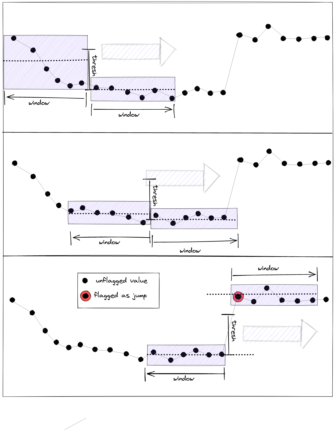
../_images/flagJumpsPic.png — The two adjacent windows of size window roll through the whole data series. Whenever the mean values in the two windows differ by more than thresh, flagging is triggered.#

Notes

Jumps that are not distanced to each other by more than three fourth (3/4) of the selected window size, will not be detected reliably.

flagLOF(field, n=20, thresh=1.5, algorithm='ball_tree', p=1, flag=255.0, **kwargs)#

Flag values where the Local Outlier Factor (LOF) exceeds cutoff.

Parameters:

field (str | list[str]) – Variable to process.
n (int (default: 20)) –
Number of neighbors to be included into the LOF calculation. Defaults to 20, which is a value found to be suitable in the literature.
- n determines the “locality” of an observation (its n nearest neighbors) and sets the upper limit to the number of values in outlier clusters (i.e. consecutive outliers). Outlier clusters of size greater than n/2 may not be detected reliably.
- The larger n, the lesser the algorithm’s sensitivity to local outliers and small or singleton outliers points. Higher values greatly increase numerical costs.
thresh (Union[Literal['auto'], float] (default: 1.5)) –
The threshold for flagging the calculated LOF. A LOF of around 1 is considered normal and most likely corresponds to inlier points.
- The “automatic” threshing introduced with the publication of the algorithm defaults to 1.5.
- In this implementation, thresh defaults ('auto') to flagging the scores with a modified 3-sigma rule.
algorithm (Literal['ball_tree', 'kd_tree', 'brute', 'auto'] (default: 'ball_tree')) – Algorithm used for calculating the n-nearest neighbors.
p (int (default: 1)) –
Degree of the metric (“Minkowski”), according to which the distance to neighbors is determined. Most important values are:
- 1 - Manhattan Metric
- 2 - Euclidian Metric
density –
How to calculate the temporal distance/density for the variable to flag.
- 'auto' - introduces linear density with an increment equal to the median of the absolute diff of the variable to flag.
- float - introduces linear density with an increment equal to density
- Callable - calculates the density by applying the function passed onto the variable to flag (passed as Series).
target (str | list[str], optional) – Variable name to which the results are written. target will be created if it does not exist. Defaults to field.
dfilter (Any, optional) – Defines which observations will be masked based on the already existing flags. Any data point with a flag equal or worse to this threshold will be passed as NaN to the function. Defaults to the DFILTER_ALL value of the translation scheme.
flag (Any, optional) – The flag value the function uses to mark observations. Defaults to the BAD value of the translation scheme.

Returns:

SaQC – the updated SaQC object

Return type:

saqc.SaQC

Notes

The flagLOF() function calculates the Local Outlier Factor (LOF) for every point in the input timeseries. The LOF is a scalar value, that roughly correlates to the reachability, or “outlierishnes” of the evaluated datapoint. If a point is as reachable, as all its n-nearest neighbors, the LOF score evaluates to around 1. If it is only as half as reachable as all its n-nearest neighbors are (so to say, as double as “outlierish”), the score is about 2. So, the Local Outlier Factor relates a point’s reachability to the reachability of its n-nearest neighbors in a multiplicative fashion (as a “factor”).
The reachability of a point thereby is determined as an aggregation of the points distances to its n-nearest neighbors, measured with regard to the minkowski metric of degree p (usually euclidean).
To derive a binary label for every point (outlier: yes, or no), the scores are cut off at a level, determined by thresh.

flagMAD(field, window=None, z=3.5, min_residuals=None, min_periods=None, center=False, flag=255.0, **kwargs)#

Flag outiers using the modified Z-score outlier detection method.

See references [1] for more details on the algorithm.

Deprecated since version 2.6.0: Deprecated Function. Please refer to flagZScore().

Parameters:

field (str | list[str]) – Variable to process.
window (UnionType[str, int, None] (default: None)) – Size of the window. Either given as an Offset String, denoting the window’s temporal extension or as an integer, denoting the window’s number of periods. NaN also count as periods. If None, all data points share the same scoring window, which than equals the whole data.
z (float (default: 3.5)) – The value the Z-score is tested against. Defaulting to 3.5 (Recommendation of [1])
min_periods (Optional[int] (default: None)) – Minimum number of valid meassurements in a scoring window, to consider the resulting score valid.
center (bool (default: False)) – Weather or not to center the target value in the scoring window. If False, the target value is the last value in the window.
target (str | list[str], optional) – Variable name to which the results are written. target will be created if it does not exist. Defaults to field.
dfilter (Any, optional) – Defines which observations will be masked based on the already existing flags. Any data point with a flag equal or worse to this threshold will be passed as NaN to the function. Defaults to the DFILTER_ALL value of the translation scheme.
flag (Any, optional) – The flag value the function uses to mark observations. Defaults to the BAD value of the translation scheme.

Returns:

SaQC – the updated SaQC object

Return type:

saqc.SaQC

Notes

Data needs to be sampled at a regular equidistant time grid.

References

[1] https://www.itl.nist.gov/div898/handbook/eda/section3/eda35h.htm

flagMVScores(field, trafo=<function OutliersMixin.<lambda>>, alpha=0.05, n=10, func='sum', iter_start=0.5, window=None, min_periods=11, stray_range=None, drop_flagged=False, thresh=3.5, min_periods_r=1, flag=255.0, **kwargs)#

The algorithm implements a 3-step outlier detection procedure for simultaneously flagging of higher dimensional data (dimensions > 3).

In [1], the procedure is introduced and exemplified with an application on hydrological data. See the notes section for an overview over the algorithms basic steps.

Deprecated since version 2.6.0: Deprecated Function. Please refer to flagByStray().

Parameters:

field (List[str]) – List of variables names to process.
trafo (Callable[[Series], Series] (default: <function OutliersMixin.<lambda> at 0x7f21149b7e20>)) – Transformation to be applied onto every column before scoring. For more fine-grained control, the data could also be transformed before flagMVScores() is called.
alpha (float (default: 0.05)) – Level of significance by which it is tested, if an observations score might be drawn from another distribution than the majority of the data.
n (int (default: 10)) – Number of neighbors included in the scoring process for every datapoint.
func (Union[Callable[[Series], float], str] (default: 'sum')) – Function that aggregates a value’s k-smallest distances, returning a scalar score.
iter_start (float (default: 0.5)) – Value in [0,1] that determines which percentage of data is considered “normal”. 0.5 results in the threshing algorithm to search only the upper 50% of the scores for the cut-off point. (See reference section for more information)
window (UnionType[int, str, None] (default: None)) – Only effective if threshing is set to 'stray'. Determines the size of the data partitions, the data is decomposed into. Each partition is checked seperately for outliers. Either given as an Offset String, denoting the windows temporal extension or as an integer, denoting the windows number of periods. NaN also count as periods. If None, all data points share the same scoring window, which than equals the whole data.
min_periods (int (default: 11)) – Only effective if threshing is set to 'stray' and partition is an integer. Minimum number of periods per partition that have to be present for a valid outlier detection to be made in this partition.
stray_range (Optional[str] (default: None)) – If not None, it is tried to reduce the stray result onto single outlier components of the input field. The offset string denotes the range of the temporal surrounding to include into the MAD testing while trying to reduce flags.
drop_flagged (bool (default: False)) – Only effective when stray_range is not None. Whether or not to drop flagged values from the temporal surroundings.
thresh (float (default: 3.5)) – Only effective when stray_range is not None. The ‘critical’ value, controlling wheather the MAD score is considered referring to an outlier or not. Higher values result in less rigid flagging. The default value is widely considered apropriate in the literature.
min_periods_r (int (default: 1)) – Only effective when stray_range is not None. Minimum number of measurements necessary in an interval to actually perform the reduction step.
target (str | list[str], optional) – Variable name to which the results are written. target will be created if it does not exist. Defaults to field.
dfilter (Any, optional) – Defines which observations will be masked based on the already existing flags. Any data point with a flag equal or worse to this threshold will be passed as NaN to the function. Defaults to the DFILTER_ALL value of the translation scheme.
flag (Any, optional) – The flag value the function uses to mark observations. Defaults to the BAD value of the translation scheme.

Returns:

SaQC – the updated SaQC object

Return type:

saqc.SaQC

Notes

The basic steps are:

transforming

The different data columns are transformed via timeseries transformations to (a) make them comparable and (b) make outliers more stand out.

This step is usually subject to a phase of research/try and error. See [1] for more details.

Note, that the data transformation as a built-in step of the algorithm, will likely get deprecated in the future. It’s better to transform the data in a processing step, preceeding the multivariate flagging process. Also, by doing so, one gets mutch more control and variety in the transformation applied, since the trafo parameter only allows for application of the same transformation to all the variables involved.

scoring

Every observation gets assigned a score depending on its k nearest neighbors. See the scoring_method parameter description for details on the different scoring methods. Furthermore, [1] may give some insight in the pro and cons of the different methods.

threshing

The gaps between the (greatest) scores are tested for beeing drawn from the same distribution as the majority of the scores. If a gap is encountered, that, with sufficient significance, can be said to not be drawn from the same distribution as the one all the smaller gaps are drawn from, than the observation belonging to this gap, and all the observations belonging to gaps larger than this gap, get flagged outliers. See description of the threshing parameter for more details. Although [1] gives a fully detailed overview over the stray algorithm.

References

[1] Priyanga Dilini Talagala, Rob J. Hyndman & Kate Smith-Miles (2021):: Anomaly Detection in High-Dimensional Data, Journal of Computational and Graphical Statistics, 30:2, 360-374, DOI: 10.1080/10618600.2020.1807997

flagManual(field, mdata, method='left-open', mformat='start-end', mflag=1, flag=255.0, **kwargs)#

Include flags listed in external data.

The method allows to integrate pre-existing flagging information.

Deprecated since version 2.6.0: Deprecated Function. See setFlags().

Parameters:

field (str | list[str]) – Variable to process.
mdata (str | Series | ndarray | list | DataFrame | DictOfSeries) –
Determines which values or intervals will be flagged. Supported input types:
- pd.Series: Needs a datetime index and values of type:
  - datetime, for method values "right-closed", "left-closed", "closed"
  - or any scalar, for method values "plain", "ontime"
- str: Variable holding the manual flag information.
- pd.DataFrame, DictOfSeries: Need to provide a pd.Series with column name field.
- list, np.ndarray: Only supported with method value "plain" and mformat value "mflag"
method (Literal['left-open', 'right-open', 'closed', 'plain', 'ontime'] (default: 'left-open')) –
Defines how mdata is projected to data:
- "plain": mdata must have the same length as field, flags are set, where the values in mdata equal mflag.
- "ontime": Expects datetime indexed mdata (types pd.Series, pd.DataFrame, DictOfSeries). Flags are set, where the values in mdata equal mflag and the indices of field and mdata match.
- "right-open": Expects datetime indexed mdata, which will be interpreted as a number of time intervals t_1, t_2. Flags are set to all timestamps t of field with t_1 <= t < t_2.
- "left-open": like "right-open", but the interval covers all t with t_1 < t <= t_2.
- "closed": like "right-open", but the interval now covers all t with t_1 <= t <= t_2.
mformat (Literal['start-end', 'mflag'] (default: 'start-end')) –
Controls the interval definition in mdata (see examples):
- "start-end": expects datetime indexed mdata (types pd.Series, pd.DataFrame, DictOfSeries) with values of type datetime. Each index-value pair is interpreted as an interval to flag, the index defines the left bound, the respective value the right bound.
- "mflag":
  - mdata of type pd.Series, pd.DataFrame, DictOfSeries: Two successive index values i_1, i_2 will be interpreted as an interval t_1, t_2 to flag, if the value of t_1 equals mflag
  - mdata of type list, np.ndarray: Flags all field where mdata euqals mflag.
mflag (Any (default: 1)) – Value in mdata indicating that a flag should be set at the respective position, timestamp or interval. Ignored if mformat is set to "start-end".
target (str | list[str], optional) – Variable name to which the results are written. target will be created if it does not exist. Defaults to field.
dfilter (Any, optional) – Defines which observations will be masked based on the already existing flags. Any data point with a flag equal or worse to this threshold will be passed as NaN to the function. Defaults to the DFILTER_ALL value of the translation scheme.
flag (Any, optional) – The flag value the function uses to mark observations. Defaults to the BAD value of the translation scheme.

Returns:

SaQC – the updated SaQC object

Return type:

saqc.SaQC

Examples

Usage of mdata

>>> import saqc
>>> mdata = pd.Series([1, 0, 1], index=pd.to_datetime(['2000-02-01', '2000-03-01', '2000-05-01']))
>>> mdata
2000-02-01    1
2000-03-01    0
2000-05-01    1
dtype: int64

On daily data, with method "ontime", only the provided timestamps are used. Only exact matches apply, offsets will be ignored.

>>> data = pd.Series(0, index=pd.to_datetime(['2000-01-31', '2000-02-01', '2000-02-02', '2000-03-01', '2000-05-01']), name='daily_data')
>>> qc = saqc.SaQC(data)
>>> qc = qc.flagManual('daily_data', mdata, mflag=1, mformat='mflag', method='ontime')
>>> qc.flags['daily_data'] > UNFLAGGED
2000-01-31    False
2000-02-01     True
2000-02-02    False
2000-03-01    False
2000-05-01     True
dtype: bool

With method "right-open" , mdata is forward filled:

>>> qc = qc.flagManual('daily_data', mdata, mflag=1, mformat='mflag', method='right-open')
>>> qc.flags['daily_data'] > UNFLAGGED
2000-01-31    False
2000-02-01     True
2000-02-02     True
2000-03-01    False
2000-05-01     True
dtype: bool

With method "left-open" , mdata is backward filled:

>>> qc = qc.flagManual('daily_data', mdata, mflag=1, mformat='mflag', method='left-open')
>>> qc.flags['daily_data'] > UNFLAGGED
2000-01-31    False
2000-02-01     True
2000-02-02     True
2000-03-01     True
2000-05-01     True
dtype: bool

flagMissing(field, flag=255.0, dfilter=-inf, **kwargs)#

Flag NaNs in data.

By default, only NaNs are flagged, that not already have a flag. dfilter can be used to pass a flag that is used as threshold. Each flag worse than the threshold is replaced by the function. This is, because the data gets masked (with NaNs) before the function evaluates the NaNs.

Parameters:

field (str | list[str]) – Variable to process.
target (str | list[str], optional) – Variable name to which the results are written. target will be created if it does not exist. Defaults to field.
dfilter (Any, optional) – Defines which observations will be masked based on the already existing flags. Any data point with a flag equal or worse to this threshold will be passed as NaN to the function. Defaults to the DFILTER_ALL value of the translation scheme.
flag (Any, optional) – The flag value the function uses to mark observations. Defaults to the BAD value of the translation scheme.

Returns:

SaQC – the updated SaQC object

Return type:

saqc.SaQC

flagOffset(field, tolerance, window, thresh=None, thresh_relative=None, flag=255.0, **kwargs)#

A basic outlier test that works on regularly and irregularly sampled data.

The test classifies values/value courses as outliers by detecting not only a rise in value, but also, by checking for a return to the initial value level.

Parameters:

field (str | list[str]) – Variable to process.
tolerance (float) – Maximum difference allowed between the value, directly preceding and the value directly succeeding an offset to trigger flagging of the offsetting values. See condition (4).
window (int | str) – Maximum length allowed for offset value courses, to trigger flagging of the offsetting values. See condition (5). Integer defined window length are only allowed for regularly sampled timeseries.
thresh (Optional[float] (default: None)) – Minimum difference between a value and its successors, to consider the successors an anomalous offset group. See condition (1). If None, condition (1) is not tested.
thresh_relative (Optional[float] (default: None)) – Minimum relative change between a value and its successors, to consider the successors an anomalous offset group. See condition (2). If None, condition (2) is not tested.
target (str | list[str], optional) – Variable name to which the results are written. target will be created if it does not exist. Defaults to field.
dfilter (Any, optional) – Defines which observations will be masked based on the already existing flags. Any data point with a flag equal or worse to this threshold will be passed as NaN to the function. Defaults to the DFILTER_ALL value of the translation scheme.
flag (Any, optional) – The flag value the function uses to mark observations. Defaults to the BAD value of the translation scheme.

Returns:

SaQC – the updated SaQC object

Return type:

saqc.SaQC

Notes

This definition of a “spike” not only includes one-value outliers, but also plateau-ish value courses.

Values \(x_n, x_{n+1}, .... , x_{n+k}\) of a timeseries \(x\) with associated timestamps \(t_n, t_{n+1}, .... , t_{n+k}\) are considered spikes, if:

\(|x_{n-1} - x_{n + s}| >\) thresh, for all \(s \in [0,1,2,...,k]\)
if thresh_relative > 0, \(x_{n + s} > x_{n - 1}*(1+\) thresh_relative \()\)
if thresh_relative < 0, \(x_{n + s} < x_{n - 1}*(1+\) thresh_relative \()\)
\(|x_{n-1} - x_{n+k+1}| <\) tolerance
\(|t_{n-1} - t_{n+k+1}| <\) window

Examples

Below picture gives an abstract interpretation of the parameter interplay in case of a positive value jump, initialising an offset course.

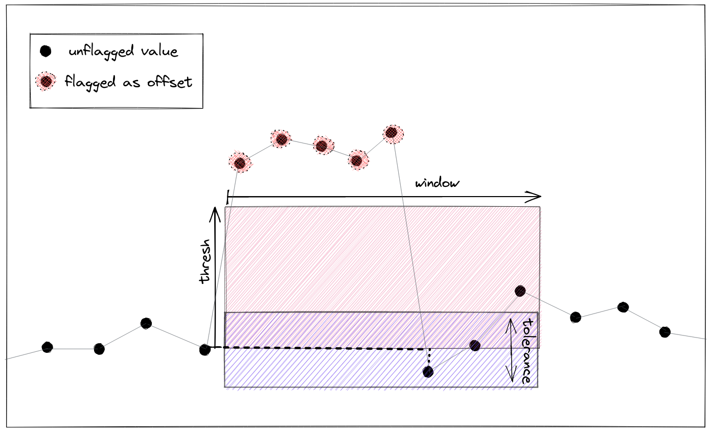
../_images/flagOffsetPic.png — The four values marked red, are flagged, because (1) the initial value jump *exceeds* the value given by `thresh`, (2) the temporal extension of the group does *not exceed* the range given by window and (3) the returning value after the group, lies *within* the value range determined by `tolerance`#

Lets generate a simple, regularly sampled timeseries with an hourly sampling rate and generate an saqc.SaQC instance from it.

>>> import saqc
>>> data = pd.DataFrame({'data':np.array([5,5,8,16,17,7,4,4,4,1,1,4])}, index=pd.date_range('2000',freq='1h', periods=12))
>>> data
                     data
2000-01-01 00:00:00     5
2000-01-01 01:00:00     5
2000-01-01 02:00:00     8
2000-01-01 03:00:00    16
2000-01-01 04:00:00    17
2000-01-01 05:00:00     7
2000-01-01 06:00:00     4
2000-01-01 07:00:00     4
2000-01-01 08:00:00     4
2000-01-01 09:00:00     1
2000-01-01 10:00:00     1
2000-01-01 11:00:00     4
>>> qc = saqc.SaQC(data)

Now we are applying flagOffset() and try to flag offset courses, that dont extend longer than 6 hours in time (window) and that have an initial value jump higher than 2 (thresh), and that do return to the initial value level within a tolerance of 1.5 (tolerance).

>>> qc = qc.flagOffset("data", thresh=2, tolerance=1.5, window='6h')
>>> qc.plot('data')  

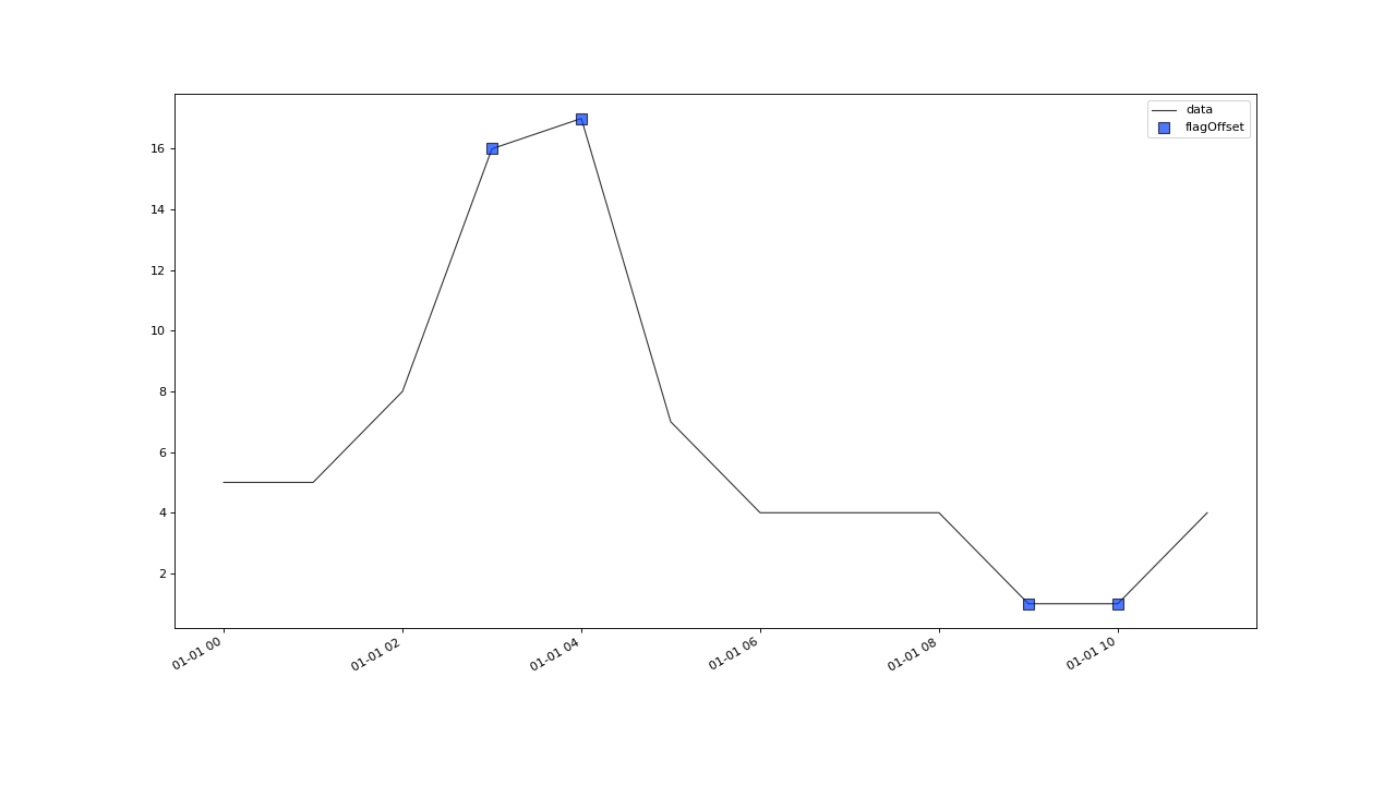
Note, that both, negative and positive jumps are considered starting points of negative or positive offsets. If you want to impose the additional condition, that the initial jump must exceed +90%* of the value level, you can additionally set the thresh_relative parameter:

>>> qc = qc.flagOffset("data", thresh=2, thresh_relative=.9, tolerance=1.5, window='6h')
>>> qc.plot('data') 

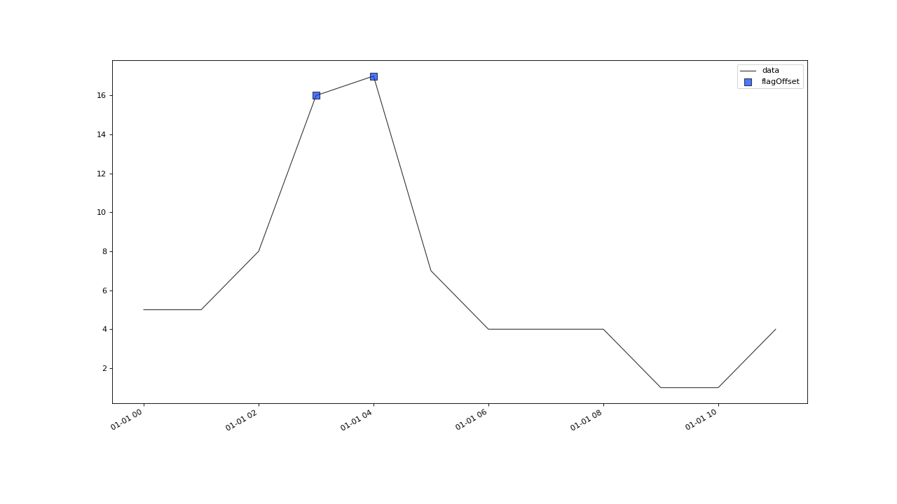
Now, only positive jumps, that exceed a value gain of +90%* are considered starting points of offsets.

In the same way, you can aim for only negative offsets, by setting a negative relative threshold. The below example only flags offsets, that fall off by at least 50% in value, with an absolute value drop of at least 2.

>>> qc = qc.flagOffset("data", thresh=2, thresh_relative=-.5, tolerance=1.5, window='6h')
>>> qc.plot('data') 

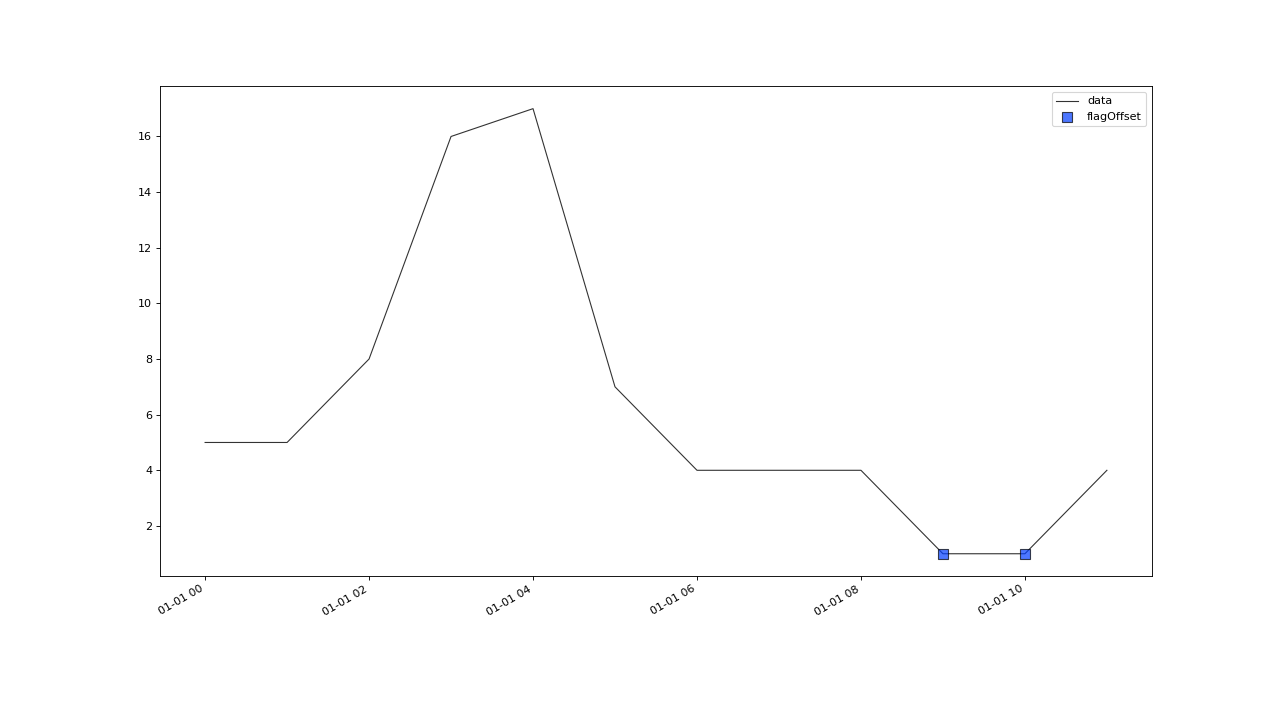
flagPatternByDTW(field, reference, max_distance=0.0, normalize=True, plot=False, flag=255.0, **kwargs)#

Pattern Recognition via Dynamic Time Warping.

The steps are: 1. work on a moving window

for each data chunk extracted from each window, a distance to the given pattern is calculated, by the dynamic time warping algorithm [1]
if the distance is below the threshold, all the data in the window gets flagged

Parameters:

field (str | list[str]) – Variable to process.
reference (str) – The name in data which holds the pattern. The pattern must not have NaNs, have a datetime index and must not be empty.
max_distance (float (default: 0.0)) – Maximum dtw-distance between chunk and pattern, if the distance is lower than max_distance the data gets flagged. With default, 0.0, only exact matches are flagged.
normalize (bool (default: True)) – If False, return unmodified distances. If True, normalize distances by the number of observations of the reference. This helps to make it easier to find a good cutoff threshold for further processing. The distances then refer to the mean distance per datapoint, expressed in the datas units.
plot (bool (default: False)) –
Show a calibration plot, which can be quite helpful to find the right threshold for max_distance. It works best with normalize=True. Do not use in automatic setups / pipelines. The plot show three lines:
- data: the data the function was called on
- distances: the calculated distances by the algorithm
- indicator: have to distinct levels: 0 and the value of max_distance. If max_distance is 0.0 it defaults to 1. Everywhere where the indicator is not 0 the data will be flagged.
target (str | list[str], optional) – Variable name to which the results are written. target will be created if it does not exist. Defaults to field.
dfilter (Any, optional) – Defines which observations will be masked based on the already existing flags. Any data point with a flag equal or worse to this threshold will be passed as NaN to the function. Defaults to the DFILTER_ALL value of the translation scheme.
flag (Any, optional) – The flag value the function uses to mark observations. Defaults to the BAD value of the translation scheme.

Returns:

SaQC – the updated SaQC object

Return type:

saqc.SaQC

Notes

The window size of the moving window is set to equal the temporal extension of the reference datas datetime index.

References

Find a nice description of underlying the Dynamic Time Warping Algorithm here:

[1] https://cran.r-project.org/web/packages/dtw/dtw.pdf

flagRaise(field, thresh, raise_window, freq, average_window=None, raise_factor=2.0, slope=None, weight=0.8, flag=255.0, **kwargs)#

The function flags raises and drops in value courses, that exceed a certain threshold within a certain timespan.

Deprecated since version 2.6.0: Function is deprecated since its not humanly parameterisable. Also more suitable alternatives are available. Depending on use case, use: flagUniLOF(), flagZScore(), flagJumps() instead.

Parameters:

field (str | list[str]) – Variable to process.
thresh (float) – The threshold, for the total rise (thresh > 0), or total drop (thresh < 0), value courses must not exceed within a timespan of length raise_window.
raise_window (str) – An offset string, determining the timespan, the rise/drop thresholding refers to. Window is inclusively defined.
freq (str) – An offset string, determining the frequency, the timeseries to flag is supposed to be sampled at. The window is inclusively defined.
average_window (Optional[str] (default: None)) – See condition (2) of the description given in the Notes. Window is inclusively defined, defaults to 1.5 times the size of raise_window.
raise_factor (float (default: 2.0)) – See condition (2).
slope (Optional[float] (default: None)) – See condition (3).
weight (float (default: 0.8)) – See condition (3).
target (str | list[str], optional) – Variable name to which the results are written. target will be created if it does not exist. Defaults to field.
dfilter (Any, optional) – Defines which observations will be masked based on the already existing flags. Any data point with a flag equal or worse to this threshold will be passed as NaN to the function. Defaults to the DFILTER_ALL value of the translation scheme.
flag (Any, optional) – The flag value the function uses to mark observations. Defaults to the BAD value of the translation scheme.

Returns:

SaQC – the updated SaQC object

Return type:

saqc.SaQC

Notes

The dataset is NOT supposed to be harmonized to a time series with an equidistant requency grid.

The value \(x_{k}\) of a time series \(x\) with associated timestamps \(t_i\), is flagged a raise, if:

There is any value \(x_{s}\), preceeding \(x_{k}\) within raise_window range, so that \(M = |x_k - x_s | >\) thresh \(> 0\)
The weighted average \(\mu^{*}\) of the values, preceding \(x_{k}\) within average_window range indicates, that \(x_{k}\) does not return from an “outlierish” value course, meaning that \(x_k > \mu^* + ( M\) / raise_factor \()\)
Additionally, if slope is not None, \(x_{k}\) is checked or being sufficiently divergent from its very predecessor \(x_{k-1}\), meaning that, it is additionally checked if: * \(x_k - x_{k-1} >\) slope * \(t_k - t_{k-1} >\) weight \(\times\) freq

flagRange(field, min=-inf, max=inf, flag=255.0, **kwargs)#

Function flags values exceeding the closed interval [min, max].

Parameters:

field (str | list[str]) – Variable to process.
min (float (default: -inf)) – Lower bound for valid data.
max (float (default: inf)) – Upper bound for valid data.
target (str | list[str], optional) – Variable name to which the results are written. target will be created if it does not exist. Defaults to field.
dfilter (Any, optional) – Defines which observations will be masked based on the already existing flags. Any data point with a flag equal or worse to this threshold will be passed as NaN to the function. Defaults to the DFILTER_ALL value of the translation scheme.
flag (Any, optional) – The flag value the function uses to mark observations. Defaults to the BAD value of the translation scheme.

Returns:

SaQC – the updated SaQC object

Return type:

saqc.SaQC

flagRegimeAnomaly(field, cluster_field, spread, method='single', metric=<function DriftMixin.<lambda>>, frac=0.5, flag=255.0, **kwargs)#

Flags anomalous regimes regarding to modelling regimes of field.

“Normality” is determined in terms of a maximum spreading distance, regimes must not exceed in respect to a certain metric and linkage method.

In addition, only a range of regimes is considered “normal”, if it models more then frac percentage of the valid samples in “field”.

Note, that you must detect the regime changepoints prior to calling this function.

Note, that it is possible to perform hypothesis tests for regime equality by passing the metric a function for p-value calculation and selecting linkage method “complete”.

Parameters:

field (str | list[str]) – Variable to process.
cluster_field (str) – Column in data, holding the cluster labels for the samples in field. (has to be indexed equal to field)
spread (float) – A threshold denoting the value level, up to wich clusters a agglomerated.
method (Literal['single', 'complete', 'average', 'weighted', 'centroid', 'median', 'ward'] (default: 'single')) – The linkage method for hierarchical (agglomerative) clustering of the variables.
metric (Callable[[ndarray | Series, ndarray | Series], float] (default: <function DriftMixin.<lambda> at 0x7f21149a74c0>)) – A metric function for calculating the dissimilarity between 2 regimes. Defaults to the absolute difference in mean.
frac (float (default: 0.5)) – The minimum percentage of samples, the “normal” group has to comprise to actually be the normal group. Must be in the closed interval [0,1], otherwise a ValueError is raised.
target (str | list[str], optional) – Variable name to which the results are written. target will be created if it does not exist. Defaults to field.
dfilter (Any, optional) – Defines which observations will be masked based on the already existing flags. Any data point with a flag equal or worse to this threshold will be passed as NaN to the function. Defaults to the DFILTER_ALL value of the translation scheme.
flag (Any, optional) – The flag value the function uses to mark observations. Defaults to the BAD value of the translation scheme.

Returns:

SaQC – the updated SaQC object

Return type:

saqc.SaQC

flagUnflagged(field, flag=255.0, **kwargs)#

Function sets a flag at all unflagged positions.

Parameters:

field (str | list[str]) – Variable to process.
target (str | list[str], optional) – Variable name to which the results are written. target will be created if it does not exist. Defaults to field.
dfilter (Any, optional) – Defines which observations will be masked based on the already existing flags. Any data point with a flag equal or worse to this threshold will be passed as NaN to the function. Defaults to the DFILTER_ALL value of the translation scheme.
flag (Any, optional) – The flag value the function uses to mark observations. Defaults to the BAD value of the translation scheme.

Returns:

SaQC – the updated SaQC object

Return type:

saqc.SaQC

Notes

This function ignores the dfilter keyword, because the data is not relevant for processing.

See also

clearFlags: set whole column to UNFLAGGED
forceFlags: set whole column to a flag value

flagUniLOF(field, n=20, thresh=1.5, algorithm='ball_tree', p=1, density='auto', fill_na=True, slope_correct=True, min_offset=None, flag=255.0, **kwargs)#

Flag “univariate” Local Outlier Factor (LOF) exceeding cutoff.

The function is a wrapper around a usual LOF implementation, aiming for an easy to use, parameter minimal outlier detection function for single variables, that does not necessitate prior modelling of the variable. LOF is applied onto a concatenation of the field variable and a “temporal density”, or “penalty” variable, that measures temporal distance between data points. See notes Section for a more exhaustive explaination. See the Notes section for more details on the algorithm.

Parameters:

field (str | list[str]) – Variable to process.
n (int (default: 20)) –
Number of periods to be included into the LOF calculation. Defaults to 20, which is a value found to be suitable in the literature.
- n determines the “locality” of an observation (its n nearest neighbors) and sets the upper limit to the number of values in an outlier clusters (i.e. consecutive outliers). Outlier clusters of size greater than n/2 may not be detected reliably.
- The larger n, the lesser the algorithm’s sensitivity to local outliers and small or singleton outlier points. Higher values greatly increase numerical costs.
thresh (Union[Literal['auto'], float] (default: 1.5)) –
The threshold for flagging the calculated LOF. A LOF of around 1 is considered normal and most likely corresponds to inlier points. This parameter is considered the main calibration parameter of the algorithm.
- The threshing defaults to 1.5, wich is the default value found to be suitable in the literature.
- 'auto' enables flagging the scores with a modified 3-sigma rule, resulting in a thresh around 4, which usually greatly mitigates overflagging compared to the literature recommendation, but often is too high.
- sensitive range for the parameter may be [1,15], assuming default settings for the other parameters.
algorithm (Literal['ball_tree', 'kd_tree', 'brute', 'auto'] (default: 'ball_tree')) – Algorithm used for calculating the n-nearest neighbors needed for LOF calculation.
p (int (default: 1)) –
Degree of the metric (“Minkowski”), according to which distance to neighbors is determined. Most important values are:
- 1 - Manhatten Metric
- 2 - Euclidian Metric
density (Union[Literal['auto'], float] (default: 'auto')) –
How to calculate the temporal distance/density for the variable to flag.
- 'auto' - introduces linear density with an increment equal to the median of the absolute diff of the variable to flag.
- float - introduces linear density with an increment equal to density
fill_na (bool (default: True)) – If True, NaNs in the data are filled with a linear interpolation.
slope_correct (bool (default: True)) – if True, a correction is applied, that removes outlier cluster that actually just seem to be steep slopes
min_offset (float (default: None)) – If set, only those outlier cluster will be flagged, that are preceeded and succeeeded by sufficiently large value “jumps”. Defaults to estimating the sufficient value jumps from the median over the absolute step sizes between data points.
target (str | list[str], optional) – Variable name to which the results are written. target will be created if it does not exist. Defaults to field.
dfilter (Any, optional) – Defines which observations will be masked based on the already existing flags. Any data point with a flag equal or worse to this threshold will be passed as NaN to the function. Defaults to the DFILTER_ALL value of the translation scheme.
flag (Any, optional) – The flag value the function uses to mark observations. Defaults to the BAD value of the translation scheme.

Returns:

SaQC – the updated SaQC object

Return type:

saqc.SaQC

Notes

The flagUniLOF() function calculates an univariate Local Outlier Factor (UniLOF) - score for every point in the one dimensional input data series. The UniLOF score of any data point is a scalar value, that roughly correlates to its reachability, or “outlierishnes” in the 2-dimensional space constituted by the data-values and the time axis. So the Algorithm basically operates on the “graph”, or the “plot” of the input timeseries.
If a point in this “graph” is as reachable, as all its n-nearest neighbors, its UniLOF score evaluates to around 1. If it is only as half as reachable as all its n neighbors are (so to say, as double as “outlierish”), its score evaluates to 2 roughly. So, the Univariate Local Outlier Factor relates a points reachability to the reachability of its n-nearest neighbors in a multiplicative fashion (as a “factor”).
The reachability of a point thereby is derived as an aggregation of the points distance to its n-nearest neighbors, measured with regard to the minkowski metric of degree p (usually euclidean).
The parameter density thereby determines how dimensionality of the time is removed, to make it a dimensionless, real valued coordinate.
To derive a binary label for every point (outlier: yes, or no), the scores are cut off at a level, determined by thresh.

Examples

See the outlier detection cookbook for a detailed introduction into the usage and tuning of the function.

Example usage with default parameter configuration:

Loading data via pandas csv file parser, casting index to DateTime, generating a SaQC instance from the data and plotting the variable representing light scattering at 254 nanometers wavelength.

>>> import saqc
>>> data = pd.read_csv('./resources/data/hydro_data.csv')
>>> data = data.set_index('Timestamp')
>>> data.index = pd.DatetimeIndex(data.index)
>>> qc = saqc.SaQC(data)
>>> qc.plot('sac254_raw') 

We apply flagUniLOF() in with default parameter values. Meaning, that the main calibration paramters n and thresh evaluate to 20 and 1.5 respectively.

>>> import saqc
>>> qc = qc.flagUniLOF('sac254_raw')
>>> qc.plot('sac254_raw') 

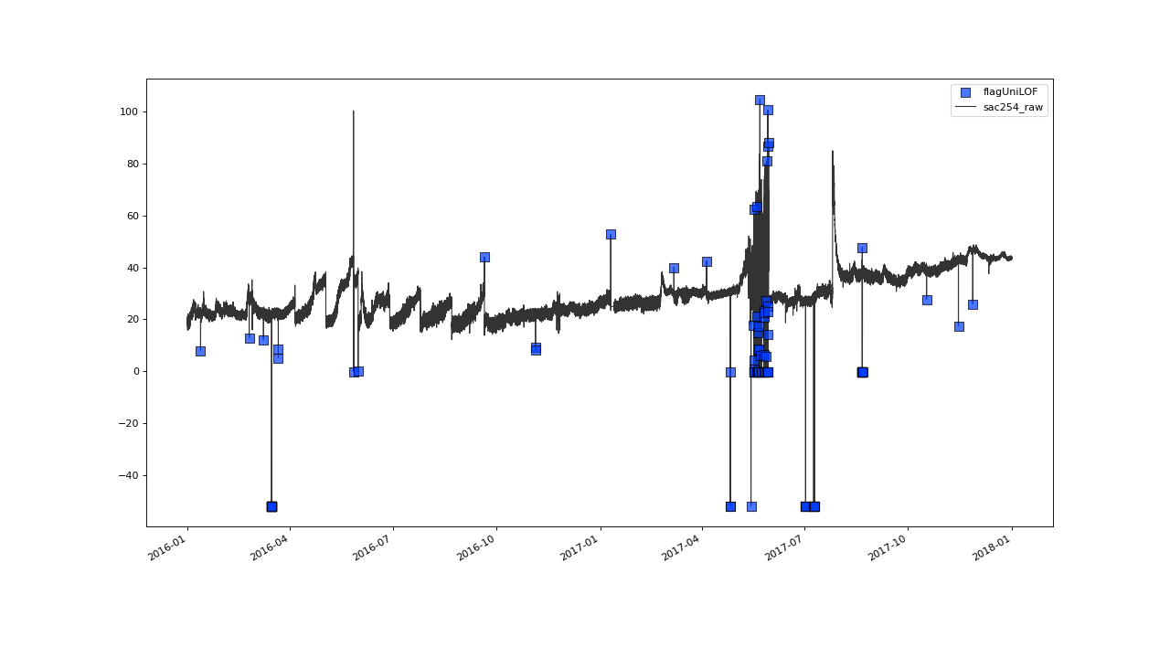
flagZScore(field, method='standard', window=None, thresh=3, min_residuals=None, min_periods=None, center=True, axis=0, flag=255.0, **kwargs)#

Flag data where its (rolling) Zscore exceeds a threshold.

The function implements flagging derived from standard or modified Zscore calculation. To handle non stationary data, the Zscoring can be applied with a rolling window. Therefor, the function allows for a minimum residual to be specified in order to mitigate overflagging in local regimes of low variance.

See the Notes section for a detailed overview of the calculation

Parameters:

field (List[str]) – List of variables names to process.
window (UnionType[str, int, None] (default: None)) – Size of the window. Either determined via an offset string, denoting the windows temporal extension or by an integer, denoting the windows number of periods. NaN also count as periods. If None is passed, all data points share the same scoring window, which than equals the whole data.
method (Literal['standard', 'modified'] (default: 'standard')) –
Which method to use for ZScoring:
- ”standard”: standard Zscoring, using mean for the expectation and standard deviation (std) as scaling factor
- ”modified”: modified Zscoring, using median as the expectation and median absolute deviation (MAD) as the scaling Factor
See notes section for detailed scoring formula
thresh (float (default: 3)) – Cutoff level for the Zscores, above which associated points are marked as outliers.
min_residuals (Optional[int] (default: None)) – Minimum residual value points must have to be considered outliers.
min_periods (Optional[int] (default: None)) – Minimum number of valid meassurements in a scoring window, to consider the resulting score valid.
center (bool (default: True)) – Weather or not to center the target value in the scoring window. If False, the target value is the last value in the window.
axis (int (default: 0)) –
Along which axis to calculate the scoring statistics:
- 0 (default) - calculate statistics along time axis
- 1 - calculate statistics over multiple variables
See Notes section for a visual clarification of the workings of axis and window.
target (str | list[str], optional) – Variable name to which the results are written. target will be created if it does not exist. Defaults to field.
dfilter (Any, optional) – Defines which observations will be masked based on the already existing flags. Any data point with a flag equal or worse to this threshold will be passed as NaN to the function. Defaults to the DFILTER_ALL value of the translation scheme.
flag (Any, optional) – The flag value the function uses to mark observations. Defaults to the BAD value of the translation scheme.

Returns:

SaQC – the updated SaQC object

Return type:

saqc.SaQC

Notes

The flag for \(x\) is determined as follows:

Depending on window and axis, the context population \(X\) is collected (see pictures below)
- If axis=0, any value is flagged in the context of those values of the same variable (field), that are in window range.
- If axis=1, any value is flagged in the context of all values of all variables (fields), that are in window range.
- If axis=0 and window=1, any value is flagged in the context of all values of all variables (fields), that share the same timestamp.

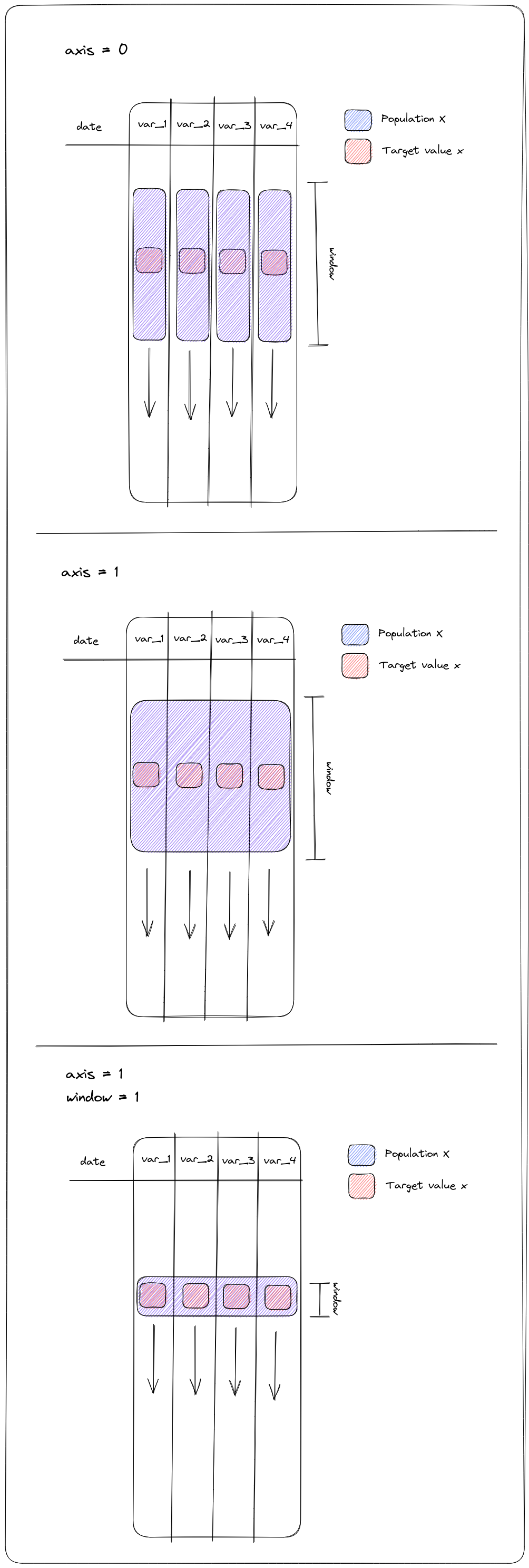
Depending on method, a score \(Z\) is calculated for \(x\) via \(Z = \frac{|E(X) - X|}{S(X)}\)
- method="standard": \(E(X)=mean(X)\), \(S(X)=std(X)\)
- method="modified": \(E(X)=median(X)\), \(S(X)=MAD(X)\)
\(x\) is flagged, if \(Z >\) thresh

forceFlags(field, flag=255.0, **kwargs)#

Set whole column to a flag value.

Parameters:: field (str | list[str]) – Variable to process.

See also

clearFlags: set whole column to UNFLAGGED
flagUnflagged: set flag value at all unflagged positions
target: str | list[str], optional Variable name to which the results are written. target will be created if it does not exist. Defaults to field.
dfilter: Any, optional Defines which observations will be masked based on the already existing flags. Any data point with a flag equal or worse to this threshold will be passed as NaN to the function. Defaults to the DFILTER_ALL value of the translation scheme.
flag: Any, optional The flag value the function uses to mark observations. Defaults to the BAD value of the translation scheme.

Returns:: SaQC – the updated SaQC object
Return type:: saqc.SaQC

interpolateByRolling(field, window, func='median', center=True, min_periods=0, flag=-inf, **kwargs)#

Replace NaN by the aggregation result of the surrounding window.

Parameters:

field (str | list[str]) – Variable to process.
window (str | int) – The size of the window, the aggregation is computed from. An integer define the number of periods to be used, a string is interpreted as an offset. ( see pandas.rolling for more information). Integer windows may result in screwed aggregations if called on none-harmonized or irregular data.
func (default median) – The function used for aggregation.
center (bool (default: True)) – Center the window around the value. Can only be used with integer windows, otherwise it is silently ignored.
min_periods (int (default: 0)) – Minimum number of valid (not np.nan) values that have to be available in a window for its aggregation to be computed.
target (str | list[str], optional) – Variable name to which the results are written. target will be created if it does not exist. Defaults to field.
dfilter (Any, optional) – Defines which observations will be masked based on the already existing flags. Any data point with a flag equal or worse to this threshold will be passed as NaN to the function. Defaults to the DFILTER_ALL value of the translation scheme.
flag (Any, optional) – The flag value the function uses to mark observations. Defaults to the BAD value of the translation scheme.

Returns:

SaQC – the updated SaQC object

Return type:

saqc.SaQC

orGroup(field, group=None, target=None, flag=255.0, **kwargs)#

Logical OR operation for Flags.

Flag the variable(s) field at every period, at wich field is flagged in at least one of the saqc objects in group.

See Examples section for examples.

Parameters:

field (str | list[str]) – Variable to process.
group (Optional[Sequence[SaQC]] (default: None)) – A collection of SaQC objects. Flag checks are performed on all SaQC objects based on the variables specified in field. Whenever any of monitored variables is flagged, the associated timestamps will receive a flag.
target (str | list[str], optional) – Variable name to which the results are written. target will be created if it does not exist. Defaults to field.
dfilter (Any, optional) – Defines which observations will be masked based on the already existing flags. Any data point with a flag equal or worse to this threshold will be passed as NaN to the function. Defaults to the DFILTER_ALL value of the translation scheme.
flag (Any, optional) – The flag value the function uses to mark observations. Defaults to the BAD value of the translation scheme.

Returns:

SaQC – the updated SaQC object

Return type:

saqc.SaQC

Examples

Flag data, if the values are above a certain threshold (determined by flagRange()) OR if the values are constant for 3 periods (determined by flagConstants())

>>> dat = pd.Series([1,0,0,0,0,2,3,4,5,5,7,8], name='data', index=pd.date_range('2000', freq='10min', periods=12))
>>> qc = saqc.SaQC(dat)
>>> qc = qc.orGroup('data', group=[qc.flagRange('data', max=5), qc.flagConstants('data', thresh=0, window=3)])
>>> qc.flags['data']
2000-01-01 00:00:00     -inf
2000-01-01 00:10:00    255.0
2000-01-01 00:20:00    255.0
2000-01-01 00:30:00    255.0
2000-01-01 00:40:00    255.0
2000-01-01 00:50:00     -inf
2000-01-01 01:00:00     -inf
2000-01-01 01:10:00     -inf
2000-01-01 01:20:00     -inf
2000-01-01 01:30:00     -inf
2000-01-01 01:40:00    255.0
2000-01-01 01:50:00    255.0
Freq: 10min, dtype: float64

plot(field, path=None, max_gap=None, mode='oneplot', history='valid', xscope=None, yscope=None, store_kwargs=None, ax=None, ax_kwargs=None, marker_kwargs=None, plot_kwargs=None, dfilter=inf, **kwargs)#

Plot data and flags or store plot to file.

There are two modes, ‘interactive’ and ‘store’, which are determined through the save_path keyword. In interactive mode (default) the plot is shown at runtime and the program execution stops until the plot window is closed manually. In store mode the generated plot is stored to disk and no manually interaction is needed.

Parameters:

field (str | list[str]) – Variable to process.
path (Optional[str] (default: None)) – If None is passed, interactive mode is entered; plots are shown immediatly and a user need to close them manually before execution continues. If a filepath is passed instead, store-mode is entered and the plot is stored unter the passed location.
max_gap (Optional[str] (default: None)) – If None, all data points will be connected, resulting in long linear lines, in case of large data gaps. NaN values will be removed before plotting. If an offset string is passed, only points that have a distance below max_gap are connected via the plotting line.
mode (Union[Literal['subplots', 'oneplot'], str] (default: 'oneplot')) –
How to process multiple variables to be plotted:
- ”oneplot” : plot all variables with their flags in one axis (default)
- ”subplots” : generate subplot grid where each axis contains one variable plot with associated flags
- ”biplot” : plotting first and second variable in field against each other in a scatter plot (point cloud).
history (Union[Literal['valid', 'complete'], list[str], None] (default: 'valid')) –
Discriminate the plotted flags with respect to the tests they originate from.
- "valid": Only plot flags, that are not overwritten by subsequent tests. Only list tests in the legend, that actually contributed flags to the overall result.
- None: Just plot the resulting flags for one variable, without any historical and/or meta information.
- list of strings: List of tests. Plot flags from the given tests, only.
- complete (not recommended, deprecated): Plot all the flags set by any test, independently from them being removed or modified by subsequent modifications. (this means: plotted flags do not necessarily match with flags ultimately assigned to the data)
xscope (UnionType[slice, str, None] (default: None)) – Determine a chunk of the data to be plotted. xscope can be anything, that is a valid argument to the pandas.Series.__getitem__ method.
yscope (UnionType[tuple, list[tuple], dict, None] (default: None)) – Either a tuple of 2 scalars that determines all plots’ y-view limits, or a list of those tuples, determining the different variables y-view limits (must match number of variables) or a dictionary with variables as keys and the y-view tuple as values.
ax (Optional[Axes] (default: None)) – If not None, plot into the given matplotlib.Axes instance, instead of a newly created matplotlib.Figure. This option offers a possibility to integrate SaQC plots into custom figure layouts.
store_kwargs (Optional[dict] (default: None)) – Keywords to be passed on to the matplotlib.pyplot.savefig method, handling the figure storing. To store an pickle object of the figure, use the option {"pickle": True}, but note that all other store_kwargs are ignored then. To reopen a pickled figure execute: pickle.load(open(savepath, "w")).show()
ax_kwargs (Optional[dict] (default: None)) –
Axis keywords. Change axis specifics. Those are passed on to the matplotlib.axes.Axes.set method and can have the options listed there. The following options are saqc specific:
- "xlabel": Either single string, that is to be attached to all x-axis´, or a List of labels, matching the number of variables to plot in length, or a dictionary, directly assigning labels to certain fields - defaults to None (no labels)
- "ylabel": Either single string, that is to be attached to all y-axis´, or a List of labels, matching the number of variables to plot in length, or a dictionary, directly assigning labels to certain fields - defaults to None (no labels)
- "title": Either a List of labels, matching the number of variables to plot in length, or a dictionary, directly assigning labels to certain variables - defaults to None (every plot gets titled the plotted variables name)
- "fontsize": (float) Adjust labeling and titeling fontsize
- "nrows", "ncols": shape of the subplot matrix the plots go into: If both are assigned, a subplot matrix of shape nrows x ncols is generated. If only one is assigned, the unassigned dimension is 1. defaults to plotting into subplot matrix with 2 columns and the necessary number of rows to fit the number of variables to plot.
marker_kwargs (Optional[dict] (default: None)) –
Keywords to modify flags marker appearance. The markers are set via the matplotlib.pyplot.scatter method and can have the options listed there. The following options are saqc specific:
- "cycleskip": (int) start the cycle of shapes that are assigned any flag-type with a certain lag - defaults to 0 (no skip)
plot_kwargs (Optional[dict] (default: None)) –
Keywords to modify the plot appearance. The plotting is delegated to matplotlib.pyplot.plot, all options listed there are available. Additionally the following saqc specific configurations are possible:
- "alpha": Either a scalar float in [0,1], that determines all plots’ transparencies, or a list of floats, matching the number of variables to plot.
- "linewidth": Either single float in [0,1], that determines the thickness of all plotted, or a list of floats, matching the number of variables to plot.
target (str | list[str], optional) – Variable name to which the results are written. target will be created if it does not exist. Defaults to field.
dfilter (Any, optional) – Defines which observations will be masked based on the already existing flags. Any data point with a flag equal or worse to this threshold will be passed as NaN to the function. Defaults to the DFILTER_ALL value of the translation scheme.
flag (Any, optional) – The flag value the function uses to mark observations. Defaults to the BAD value of the translation scheme.

Returns:

SaQC – the updated SaQC object

Return type:

saqc.SaQC

Notes

Check/modify the module parameter saqc.lib.plotting.SCATTER_KWARGS to see/modify global marker defaults
Check/modify the module parameter saqc.lib.plotting.PLOT_KWARGS to see/modify global plot line defaults

processGeneric(field, func, target=None, dfilter=-inf, **kwargs)#

Generate/process data with user defined functions.

Call the given func on the variables given in field.

Parameters:

field (str | list[str]) – Variable to process.
func (GenericFunction) – Function to call on the variables given in field. The return value will be written to target or field if the former is not given. This implies, that the function needs to accept the same number of arguments (of type pandas.Series) as variables given in field and should return an iterable of array-like objects with the same number of elements as given in target (or field if target is not specified).
target (str | list[str], optional) – Variable name to which the results are written. target will be created if it does not exist. Defaults to field.
dfilter (Any, optional) – Defines which observations will be masked based on the already existing flags. Any data point with a flag equal or worse to this threshold will be passed as NaN to the function. Defaults to the DFILTER_ALL value of the translation scheme.
flag (Any, optional) – The flag value the function uses to mark observations. Defaults to the BAD value of the translation scheme.

Returns:

SaQC – the updated SaQC object

Return type:

saqc.SaQC

Notes

All the numpy functions are available within the generic expressions.

Examples

Compute the sum of the variables ‘rainfall’ and ‘snowfall’ and save the result to a (new) variable ‘precipitation’

Examples

rainfall snowfall precipitation

1970-01-01 1 2 3

propagateFlags(field, window, method='ffill', flag=255.0, dfilter=-inf, **kwargs)#

Flag values before or after flags set by the last test.

Parameters:

field (str | list[str]) – Variable to process.
window (str | int) – Size of the repetition window. An integer defines the exact number of repetitions, strings are interpreted as time offsets to fill with.
method (Literal['ffill', 'bfill'] (default: 'ffill')) – Direction of repetetion. With “ffill” the subsequent values receive the flag to repeat, with “bfill” the previous values.
target (str | list[str], optional) – Variable name to which the results are written. target will be created if it does not exist. Defaults to field.
dfilter (Any, optional) – Defines which observations will be masked based on the already existing flags. Any data point with a flag equal or worse to this threshold will be passed as NaN to the function. Defaults to the DFILTER_ALL value of the translation scheme.
flag (Any, optional) – The flag value the function uses to mark observations. Defaults to the BAD value of the translation scheme.

Returns:

SaQC – the updated SaQC object

Return type:

saqc.SaQC

Examples

First, generate some data and some flags:

>>> import saqc
>>> data = pd.DataFrame({"a": [-3, -2, -1, 0, 1, 2, 3]})
>>> flags = pd.DataFrame({"a": [-np.inf, -np.inf, -np.inf, 255.0, -np.inf, -np.inf, -np.inf]})
>>> qc = saqc.SaQC(data=data, flags=flags)
>>> qc.flags["a"]
0     -inf
1     -inf
2     -inf
3    255.0
4     -inf
5     -inf
6     -inf
dtype: float64

Now, to repeat the flag ‘255.0’ two times in direction of ascending indices, execute:

>>> qc.propagateFlags('a', window=2, method="ffill").flags["a"]
   -inf
   -inf
   -inf
  255.0
  255.0
  255.0
   -inf
dtype: float64

Choosing “bfill” will result in

>>> qc.propagateFlags('a', window=2, method="bfill").flags["a"]
   -inf
  255.0
  255.0
  255.0
   -inf
   -inf
   -inf
dtype: float64

If an explicit flag is passed, it will be used to fill the repetition window

>>> qc.propagateFlags('a', window=2, method="bfill", flag=111).flags["a"]
   -inf
  111.0
  111.0
  255.0
   -inf
   -inf
   -inf
dtype: float64

reindex(field, index, method='match', tolerance=None, data_aggregation=None, flags_aggregation=None, broadcast=True, squeeze=False, override=False, **kwargs)#

Change a variables index.

Simultaneously changes the indices of the data, flags and the history assigned to field.

Parameters:

field (str | list[str]) – Variable to process.
index (str | DatetimeIndex) –
Determines the new index.
- If an offset string: new index will range from start to end of the original index of field, exhibting a uniform sampling rate of idx
- If a str that matches a field present in the SaQC object, that fields index will be used as new index of field
- If an pd.index object is passed, that will be the new index of field.
method (Literal['fagg', 'bagg', 'nagg', 'froll', 'broll', 'nroll', 'fshift', 'bshift', 'nshift', 'match', 'sshift', 'mshift', 'invert'] (default: 'match')) –
Determines which of the origins indexes periods to comprise into the calculation of a new flag and a new data value at any period of the new index.
- Aggregations Reindexer. Aggregations are data and flags independent, (pure) index selection methods:
- ’bagg’/’fagg’: “backwards/forwards aggregation”. Any new index period gets assigned an aggregation of the values at periods in the original index, that lie between itself and its successor/predecessor.
- ’nagg’: “nearest aggregation”: Any new index period gets assigned an aggregation of the values at periods in the original index between its direcet predecessor and successor, it is the nearest neighbor to.
- Rolling reindexer. Rolling reindexers are equal to aggregations, when projecting between regular and irregular sampling grids forth and back. But due to there simple rolling window construction, they are easier to comprehend, predict and parametrize. On the downside, they are much more expensive computationally and Also, periods can get included in the aggregation to multpiple target periods, (when rolling windows overlap).
- ’broll’/’froll’: Any new index period gets assigned an aggregation of all the values at periods of the original index, that fall into a directly preceeding/succeeding window of size reindex_window.
- Shifts. Shifting methods are shortcuts for aggregation reindex methods, combined with selecting ‘last’ or ‘first’ as the data_aggregation method. Therefor, both, the flags_aggregation and the data_aggregation are ignored when using a shift reindexer. Also, periods where the data evaluates to NaN are dropped before shift index selection.
- ’bshift’/fshift: “backwards/forwards shift”. Any new index period gets assigned the first/last valid (not a data NaN) value it succeeds/preceeds
- ’nshift’: “nearest shift”: Any new index period gets assigned the value of its closest neighbor in the original index.
- Pillar point Mappings. Index selection method designed to select indices suitable for linearly interpolating index values from surrounding pillar points in the original index, or inverting such a selection. Periods where the data evaluates to NaN, are dropped from consideration.
- ’mshift’: “Merge” predecessors and successors. Any new index period gets assigned an aggregation/interpolation comprising the last and the next valid period in the original index.
- ’sshift’: “Split”-map values onto predecessors and successors. Same as mshift, but with a correction that prevents missing value flags from being mapped to continuous data chunk bounds.
- Inversion of last method: try to select the method, that
- ’invert`
tolerance (str (default: None)) – Limiting the distance, values can be shifted or comprised into aggregation.
data_aggregation (Union[Literal['sum', 'mean', 'median', 'min', 'max', 'last', 'first', 'std', 'var', 'count', 'sem', 'linear', 'time'], Callable, float] (default: None)) – Function string or custom Function, determining how to aggregate new data values from the values at the periods selected according to the index_selection_method. If a scalar value is passed, the new data series will just evaluate to that scalar at any new index.
flags_aggregation (Union[Literal['sum', 'mean', 'median', 'min', 'max', 'last', 'first', 'std', 'var', 'count', 'sem', 'linear', 'time'], Callable, float] (default: None)) – Function string or custom Function, determining how to aggregate new flags values from the values at the periods selected according to the index_selection_method. If a scalar value is passed, the new flags series will just evaluate to that scalar at any new index.
broadcast (bool (default: True)) – Weather to propagate aggregation result to full reindex window when using aggregation reindexer. (as opposed to only assign to next/previous/closest)
target (str | list[str]) – Variable name to which the results are written. target will be created if it does not exist. Defaults to field.
dfilter (Any, optional) – Defines which observations will be masked based on the already existing flags. Any data point with a flag equal or worse to this threshold will be passed as NaN to the function. Defaults to the DFILTER_ALL value of the translation scheme.
flag (Any, optional) – The flag value the function uses to mark observations. Defaults to the BAD value of the translation scheme.

Returns:

SaQC – the updated SaQC object

Return type:

saqc.SaQC

Notes

Examples

Generate some example data with messed up 1 day-ish sampling rate

>>> import pandas as pd
>>> import saqc
>>> import numpy as np
>>> from saqc.constants import FILTER_NONE
>>> np.random.seed(23)
>>> index = pd.DatetimeIndex(pd.date_range('2000', freq='1d', periods=23))
>>> index += pd.Index([pd.Timedelta(f'{k}min') for k in np.random.randint(-360,360,23)])
>>> drops = np.random.randint(0,20,3)
>>> drops.sort()
>>> index=index[np.r_[0:drops[0],drops[0]+1:drops[1],drops[1]+1:drops[2],drops[2]+1:23]]
>>> data = pd.Series(np.abs(np.arange(-10,10)), index=index, name='data')
>>> data 
2000-01-01 03:55:00    10
2000-01-03 02:08:00     9
2000-01-03 18:31:00     8
2000-01-04 21:57:00     7
2000-01-06 01:40:00     6
2000-01-06 23:47:00     5
2000-01-09 04:02:00     4
2000-01-10 05:05:00     3
2000-01-10 18:06:00     2
2000-01-12 01:09:00     1
2000-01-13 02:44:00     0
2000-01-13 18:49:00     1
2000-01-15 05:46:00     2
2000-01-16 01:39:00     3
2000-01-17 05:49:00     4
2000-01-17 21:12:00     5
2000-01-18 18:12:00     6
2000-01-21 03:20:00     7
2000-01-21 22:57:00     8
2000-01-23 03:51:00     9
Name: data, dtype: int64

Performing linear alignment to 2 days grid, with and without limiting the reindexing range:

>>> qc = saqc.SaQC(data)
>>> qc = qc.reindex('data', target='linear', index='2D', method='mshift', data_aggregation='linear')
>>> qc = qc.reindex('data', target='limited_linear', index='2D', method='mshift', data_aggregation='linear', tolerance='1D')
>>> qc.data 
                   data |               linear |       limited_linear |
======================= | ==================== | ==================== |
2000-01-01 03:55:00  10 | 1999-12-31       NaN | 1999-12-31       NaN |
2000-01-03 02:08:00   9 | 2000-01-02  9.565453 | 2000-01-02       NaN |
2000-01-03 18:31:00   8 | 2000-01-04  7.800122 | 2000-01-04  7.800122 |
2000-01-04 21:57:00   7 | 2000-01-06  6.060132 | 2000-01-06       NaN |
2000-01-06 01:40:00   6 | 2000-01-08  4.536523 | 2000-01-08       NaN |
2000-01-06 23:47:00   5 | 2000-01-10  3.202927 | 2000-01-10  3.202927 |
2000-01-09 04:02:00   4 | 2000-01-12  1.037037 | 2000-01-12       NaN |
2000-01-10 05:05:00   3 | 2000-01-14  1.148307 | 2000-01-14       NaN |
2000-01-10 18:06:00   2 | 2000-01-16  2.917016 | 2000-01-16  2.917016 |
2000-01-12 01:09:00   1 | 2000-01-18  5.133333 | 2000-01-18  5.133333 |
2000-01-13 02:44:00   0 | 2000-01-20  6.521587 | 2000-01-20       NaN |
2000-01-13 18:49:00   1 | 2000-01-22  8.036332 | 2000-01-22       NaN |
2000-01-15 05:46:00   2 | 2000-01-24       NaN | 2000-01-24       NaN |
2000-01-16 01:39:00   3 |                      |                      |
2000-01-17 05:49:00   4 |                      |                      |
2000-01-17 21:12:00   5 |                      |                      |
2000-01-18 18:12:00   6 |                      |                      |
2000-01-21 03:20:00   7 |                      |                      |
2000-01-21 22:57:00   8 |                      |                      |
2000-01-23 03:51:00   9 |                      |                      |

Setting a flag, reindexing the linearly aligned field with the originl index (deharmonisation”)

>>> qc = qc.setFlags('linear', data=['2000-01-16'])
>>> qc = qc.reindex('linear', index='data', tolerance='2D', method='sshift', dfilter=FILTER_NONE)
>>> qc.flags[['data', 'linear']] 
                    data |                     linear |
======================== | ========================== |
2000-01-01 03:55:00 -inf | 2000-01-01 03:55:00   -inf |
2000-01-03 02:08:00 -inf | 2000-01-03 02:08:00   -inf |
2000-01-03 18:31:00 -inf | 2000-01-03 18:31:00   -inf |
2000-01-04 21:57:00 -inf | 2000-01-04 21:57:00   -inf |
2000-01-06 01:40:00 -inf | 2000-01-06 01:40:00   -inf |
2000-01-06 23:47:00 -inf | 2000-01-06 23:47:00   -inf |
2000-01-09 04:02:00 -inf | 2000-01-09 04:02:00   -inf |
2000-01-10 05:05:00 -inf | 2000-01-10 05:05:00   -inf |
2000-01-10 18:06:00 -inf | 2000-01-10 18:06:00   -inf |
2000-01-12 01:09:00 -inf | 2000-01-12 01:09:00   -inf |
2000-01-13 02:44:00 -inf | 2000-01-13 02:44:00   -inf |
2000-01-13 18:49:00 -inf | 2000-01-13 18:49:00   -inf |
2000-01-15 05:46:00 -inf | 2000-01-15 05:46:00  255.0 |
2000-01-16 01:39:00 -inf | 2000-01-16 01:39:00  255.0 |
2000-01-17 05:49:00 -inf | 2000-01-17 05:49:00   -inf |
2000-01-17 21:12:00 -inf | 2000-01-17 21:12:00   -inf |
2000-01-18 18:12:00 -inf | 2000-01-18 18:12:00   -inf |
2000-01-21 03:20:00 -inf | 2000-01-21 03:20:00   -inf |
2000-01-21 22:57:00 -inf | 2000-01-21 22:57:00   -inf |
2000-01-23 03:51:00 -inf | 2000-01-23 03:51:00   -inf |

Now, linear flags can easily be appended to data, to complete “deharm” step.

Another example: Shifting to nearest regular frequeny and back. Note, how ‘nearest’ - style reindexers “invert” themselfs.

>>> qc = saqc.SaQC(data)
>>> qc = qc.reindex('data', index='1D', target='n_shifted', method='nshift')
>>> qc = qc.reindex('n_shifted', index='data', target='n_shifted_undone', method='nshift')
>>> qc.data 
                   data |        n_shifted |          n_shifted_undone |
======================= | ================ | ========================= |
2000-01-01 03:55:00  10 | 2000-01-01  10.0 | 2000-01-01 03:55:00  10.0 |
2000-01-03 02:08:00   9 | 2000-01-02   NaN | 2000-01-03 02:08:00   9.0 |
2000-01-03 18:31:00   8 | 2000-01-03   9.0 | 2000-01-03 18:31:00   8.0 |
2000-01-04 21:57:00   7 | 2000-01-04   8.0 | 2000-01-04 21:57:00   7.0 |
2000-01-06 01:40:00   6 | 2000-01-05   7.0 | 2000-01-06 01:40:00   6.0 |
2000-01-06 23:47:00   5 | 2000-01-06   6.0 | 2000-01-06 23:47:00   5.0 |
2000-01-09 04:02:00   4 | 2000-01-07   5.0 | 2000-01-09 04:02:00   4.0 |
2000-01-10 05:05:00   3 | 2000-01-08   NaN | 2000-01-10 05:05:00   3.0 |
2000-01-10 18:06:00   2 | 2000-01-09   4.0 | 2000-01-10 18:06:00   2.0 |
2000-01-12 01:09:00   1 | 2000-01-10   3.0 | 2000-01-12 01:09:00   1.0 |
2000-01-13 02:44:00   0 | 2000-01-11   2.0 | 2000-01-13 02:44:00   0.0 |
2000-01-13 18:49:00   1 | 2000-01-12   1.0 | 2000-01-13 18:49:00   1.0 |
2000-01-15 05:46:00   2 | 2000-01-13   0.0 | 2000-01-15 05:46:00   2.0 |
2000-01-16 01:39:00   3 | 2000-01-14   1.0 | 2000-01-16 01:39:00   3.0 |
2000-01-17 05:49:00   4 | 2000-01-15   2.0 | 2000-01-17 05:49:00   4.0 |
2000-01-17 21:12:00   5 | 2000-01-16   3.0 | 2000-01-17 21:12:00   5.0 |
2000-01-18 18:12:00   6 | 2000-01-17   4.0 | 2000-01-18 18:12:00   6.0 |
2000-01-21 03:20:00   7 | 2000-01-18   5.0 | 2000-01-21 03:20:00   7.0 |
2000-01-21 22:57:00   8 | 2000-01-19   6.0 | 2000-01-21 22:57:00   8.0 |
2000-01-23 03:51:00   9 | 2000-01-20   NaN | 2000-01-23 03:51:00   9.0 |
                        | 2000-01-21   7.0 |                           |
                        | 2000-01-22   8.0 |                           |
                        | 2000-01-23   9.0 |                           |
                        | 2000-01-24   NaN |                           |

Furthermoer, forward/backward style reindexers can be inverted by backward/forward style reindexers:

>>> qc = saqc.SaQC(data)
>>> qc = qc.reindex('data', target='sum_aggregate', index='3D', method='fagg', data_aggregation='sum')
>>> qc = qc.setFlags('sum_aggregate', data=['2000-01-18', '2000-01-24'])
>>> qc = qc.reindex('sum_aggregate', target='bagg', index='data', method='bagg', dfilter=FILTER_NONE)
>>> qc = qc.reindex('sum_aggregate', target='bagg_limited', index='data', method='bagg', tolerance='2D', dfilter=FILTER_NONE)
>>> qc.flags 
                    data |     sum_aggregate |                       bagg |               bagg_limited |
======================== | ================= | ========================== | ========================== |
2000-01-01 03:55:00 -inf | 1999-12-31   -inf | 2000-01-01 03:55:00   -inf | 2000-01-01 03:55:00   -inf |
2000-01-03 02:08:00 -inf | 2000-01-03   -inf | 2000-01-03 02:08:00   -inf | 2000-01-03 02:08:00   -inf |
2000-01-03 18:31:00 -inf | 2000-01-06   -inf | 2000-01-03 18:31:00   -inf | 2000-01-03 18:31:00   -inf |
2000-01-04 21:57:00 -inf | 2000-01-09   -inf | 2000-01-04 21:57:00   -inf | 2000-01-04 21:57:00   -inf |
2000-01-06 01:40:00 -inf | 2000-01-12   -inf | 2000-01-06 01:40:00   -inf | 2000-01-06 01:40:00   -inf |
2000-01-06 23:47:00 -inf | 2000-01-15   -inf | 2000-01-06 23:47:00   -inf | 2000-01-06 23:47:00   -inf |
2000-01-09 04:02:00 -inf | 2000-01-18  255.0 | 2000-01-09 04:02:00   -inf | 2000-01-09 04:02:00   -inf |
2000-01-10 05:05:00 -inf | 2000-01-21   -inf | 2000-01-10 05:05:00   -inf | 2000-01-10 05:05:00   -inf |
2000-01-10 18:06:00 -inf | 2000-01-24  255.0 | 2000-01-10 18:06:00   -inf | 2000-01-10 18:06:00   -inf |
2000-01-12 01:09:00 -inf |                   | 2000-01-12 01:09:00   -inf | 2000-01-12 01:09:00   -inf |
2000-01-13 02:44:00 -inf |                   | 2000-01-13 02:44:00   -inf | 2000-01-13 02:44:00   -inf |
2000-01-13 18:49:00 -inf |                   | 2000-01-13 18:49:00   -inf | 2000-01-13 18:49:00   -inf |
2000-01-15 05:46:00 -inf |                   | 2000-01-15 05:46:00  255.0 | 2000-01-15 05:46:00   -inf |
2000-01-16 01:39:00 -inf |                   | 2000-01-16 01:39:00  255.0 | 2000-01-16 01:39:00  255.0 |
2000-01-17 05:49:00 -inf |                   | 2000-01-17 05:49:00  255.0 | 2000-01-17 05:49:00  255.0 |
2000-01-17 21:12:00 -inf |                   | 2000-01-17 21:12:00  255.0 | 2000-01-17 21:12:00  255.0 |
2000-01-18 18:12:00 -inf |                   | 2000-01-18 18:12:00   -inf | 2000-01-18 18:12:00   -inf |
2000-01-21 03:20:00 -inf |                   | 2000-01-21 03:20:00  255.0 | 2000-01-21 03:20:00   -inf |
2000-01-21 22:57:00 -inf |                   | 2000-01-21 22:57:00  255.0 | 2000-01-21 22:57:00   -inf |
2000-01-23 03:51:00 -inf |                   | 2000-01-23 03:51:00  255.0 | 2000-01-23 03:51:00  255.0 |

renameField(field, new_name, **kwargs)#

Rename field in data and flags.

Parameters:

field (str | list[str]) – Variable to process.
new_name (str) – String, field is to be replaced with.
target (str | list[str], optional) – Variable name to which the results are written. target will be created if it does not exist. Defaults to field.
dfilter (Any, optional) – Defines which observations will be masked based on the already existing flags. Any data point with a flag equal or worse to this threshold will be passed as NaN to the function. Defaults to the DFILTER_ALL value of the translation scheme.
flag (Any, optional) – The flag value the function uses to mark observations. Defaults to the BAD value of the translation scheme.

Returns:

SaQC – the updated SaQC object

Return type:

saqc.SaQC

resample(field, freq, func='mean', method='bagg', maxna=None, maxna_group=None, squeeze=False, **kwargs)#

Resample data points and flags to a regular frequency.

The data will be sampled to regular (equidistant) timestamps. Sampling intervals therefore get aggregated with a function, specified by func, the result is projected to the new timestamps using method. The following methods are available:

'nagg': all values in the range (+/- freq/2) of a grid point get aggregated with func and assigned to it.
'bagg': all values in a sampling interval get aggregated with func and the result gets assigned to the last grid point.
'fagg': all values in a sampling interval get aggregated with func and the result gets assigned to the next grid point.

Parameters:

field (str | list[str]) – Variable to process.
freq (str) – Offset string. Sampling rate of the target frequency grid.
func (Union[Callable[[Series], Series], str] (default: 'mean')) – Aggregation function. See notes for performance considerations.
method (Literal['fagg', 'bagg', 'nagg'] (default: 'bagg')) – Specifies which intervals to be aggregated for a certain timestamp. (preceding, succeeding or “surrounding” interval). See description above for more details.
maxna (Optional[int] (default: None)) – Maximum number of allowed NaN``s in a resampling interval. If exceeded, the aggregation of the interval evaluates to ``NaN.
maxna_group (Optional[int] (default: None)) – Same as maxna but for consecutive NaNs.
target (str | list[str], optional) – Variable name to which the results are written. target will be created if it does not exist. Defaults to field.
dfilter (Any, optional) – Defines which observations will be masked based on the already existing flags. Any data point with a flag equal or worse to this threshold will be passed as NaN to the function. Defaults to the DFILTER_ALL value of the translation scheme.
flag (Any, optional) – The flag value the function uses to mark observations. Defaults to the BAD value of the translation scheme.

Returns:

SaQC – the updated SaQC object

Return type:

saqc.SaQC

Notes

For perfomance reasons, func will be mapped to pandas.resample methods, if possible. However, for this to work, functions need an initialized __name__ attribute, holding the function’s name. Furthermore, you should not pass numpys nan-functions (nansum, nanmean,…) because they cannot be optimised and the handling of NaN is already taken care of.

rolling(field, window, target=None, func='mean', min_periods=0, center=True, **kwargs)#

Calculate a rolling-window function on the data.

Note, that the new data gets assigned the worst flag present in the window it was aggregated from.

Note, That you also can select multiple fields to get a rolling calculation over those.

Parameters:

field (str | list[str]) – Variable to process.
window (str | int) – The size of the window you want to roll with. If an integer is passed, the size refers to the number of periods for every fitting window. If an offset string is passed, the size refers to the total temporal extension. For regularly sampled timeseries, the period number will be casted down to an odd number if center=True.
func (default mean) – Function to roll with.
min_periods (int (default: 0)) – The minimum number of periods to get a valid value
center (bool (default: True)) – If True, center the rolling window.
target (str | list[str], optional) – Variable name to which the results are written. target will be created if it does not exist. Defaults to field.
dfilter (Any, optional) – Defines which observations will be masked based on the already existing flags. Any data point with a flag equal or worse to this threshold will be passed as NaN to the function. Defaults to the DFILTER_ALL value of the translation scheme.
flag (Any, optional) – The flag value the function uses to mark observations. Defaults to the BAD value of the translation scheme.

Returns:

SaQC – the updated SaQC object

Return type:

saqc.SaQC

Notes

../_images/horizontalAxisRollingExample.png — Rolling over multiple variables.#

selectTime(field, mode, selection_field=None, start=None, end=None, closed=True, **kwargs)#

Realizes masking within saqc.

Due to some inner saqc mechanics, it is not straight forwardly possible to exclude values or datachunks from flagging routines. This function replaces flags with UNFLAGGED value, wherever values are to get masked. Furthermore, the masked values get replaced by np.nan, so that they dont effect calculations.

Here comes a recipe on how to apply a flagging function only on a masked chunk of the variable field:

dublicate “field” in the input data (copyField)
mask the dublicated data (this, selectTime)
apply the tests you only want to be applied onto the masked data chunks (a saqc function)
project the flags, calculated on the dublicated and masked data onto the original field data (concateFlags or flagGeneric)
drop the dublicated data (dropField)

To see an implemented example, checkout flagSeasonalRange in the saqc.functions module

Parameters:

field (str | list[str]) – Variable to process.
mode (Literal['periodic', 'selection_field']) – The masking mode. - “periodic”: parameters “period_start”, “end” are evaluated to generate a periodical mask - “mask_var”: data[mask_var] is expected to be a boolean valued timeseries and is used as mask.
selection_field (Optional[str] (default: None)) – Only effective if mode == “mask_var” Fieldname of the column, holding the data that is to be used as mask. (must be boolean series) Neither the series` length nor its labels have to match data[field]`s index and length. An inner join of the indices will be calculated and values get masked where the values of the inner join are True.
start (Optional[str] (default: None)) – Only effective if mode == “seasonal” String denoting starting point of every period. Formally, it has to be a truncated instance of “mm-ddTHH:MM:SS”. Has to be of same length as end parameter. See examples section below for some examples.
end (Optional[str] (default: None)) – Only effective if mode == “periodic” String denoting starting point of every period. Formally, it has to be a truncated instance of “mm-ddTHH:MM:SS”. Has to be of same length as end parameter. See examples section below for some examples.
closed (bool (default: True)) – Wheather or not to include the mask defining bounds to the mask.
target (str | list[str], optional) – Variable name to which the results are written. target will be created if it does not exist. Defaults to field.
dfilter (Any, optional) – Defines which observations will be masked based on the already existing flags. Any data point with a flag equal or worse to this threshold will be passed as NaN to the function. Defaults to the DFILTER_ALL value of the translation scheme.
flag (Any, optional) – The flag value the function uses to mark observations. Defaults to the BAD value of the translation scheme.

Returns:

SaQC – the updated SaQC object

Return type:

saqc.SaQC

Examples

The period_start and end parameters provide a conveniant way to generate seasonal / date-periodic masks. They have to be strings of the forms:

“mm-ddTHH:MM:SS”
“ddTHH:MM:SS”
“HH:MM:SS”
“MM:SS” or “SS”

(mm=month, dd=day, HH=hour, MM=minute, SS=second) Single digit specifications have to be given with leading zeros. period_start and seas on_end strings have to be of same length (refer to the same periodicity) The highest date unit gives the period. For example:

>>> start = "01T15:00:00"
>>> end = "13T17:30:00"

Will result in all values sampled between 15:00 at the first and 17:30 at the 13th of every month get masked

>>> start = "01:00"
>>> end = "04:00"

All the values between the first and 4th minute of every hour get masked.

>>> start = "01-01T00:00:00"
>>> end = "01-03T00:00:00"

Mask january and february of evcomprosed in theery year. masking is inclusive always, so in this case the mask will include 00:00:00 at the first of march. To exclude this one, pass:

>>> start = "01-01T00:00:00"
>>> end = "02-28T23:59:59"

To mask intervals that lap over a seasons frame, like nights, or winter, exchange sequence of season start and season end. For example, to mask night hours between 22:00:00 in the evening and 06:00:00 in the morning, pass:

>> start = “22:00:00” >> end = “06:00:00”

setFlags(field, data, override=False, flag=255.0, **kwargs)#

Include flags listed in external data.

Parameters:

field (str | list[str]) – Variable to process.
data (str | list | ndarray | Series) –
Determines which timestamps to set flags at, depending on the passed type:
- 1-d array or List of timestamps or pandas.Index: flag field with flag at every timestamp in f_data
- 2-d array or List of tuples: for all elements t[k] out of f_data: flag field with flag at every timestamp in between t[k][0] and t[k][1]
- pd.Series: flag field with flag in between any index and data value of the passed series
- str: use the variable timeseries f_data as flagging template
- pd.Series: flag field with flag in between any index and data value of the passed series
- 1-d array or List of timestamps: flag field with flag at every timestamp in f_data
- 2-d array or List of tuples: for all elements t[k] out of f_data: flag field with flag at every timestamp in between t[k][0] and t[k][1]
override (bool (default: False)) – determines if flags shall be assigned although the value in question already has a flag assigned.
target (str | list[str], optional) – Variable name to which the results are written. target will be created if it does not exist. Defaults to field.
dfilter (Any, optional) – Defines which observations will be masked based on the already existing flags. Any data point with a flag equal or worse to this threshold will be passed as NaN to the function. Defaults to the DFILTER_ALL value of the translation scheme.
flag (Any, optional) – The flag value the function uses to mark observations. Defaults to the BAD value of the translation scheme.

Returns:

SaQC – the updated SaQC object

Return type:

saqc.SaQC

transferFlags(field, target=None, squeeze=False, overwrite=False, **kwargs)#

Transfer Flags of one variable to another.

Parameters:

field (str | list[str]) – Variable to process.
squeeze (bool (default: False)) – Squeeze the history into a single column if True, function specific flag information is lost.
overwrite (bool (default: False)) – Overwrite existing flags if True.
target (str | list[str], optional) – Variable name to which the results are written. target will be created if it does not exist. Defaults to field.
dfilter (Any, optional) – Defines which observations will be masked based on the already existing flags. Any data point with a flag equal or worse to this threshold will be passed as NaN to the function. Defaults to the DFILTER_ALL value of the translation scheme.
flag (Any, optional) – The flag value the function uses to mark observations. Defaults to the BAD value of the translation scheme.

Returns:

SaQC – the updated SaQC object

Return type:

saqc.SaQC

Examples

First, generate some data with some flags:

>>> import saqc
>>> data = pd.DataFrame({'a': [1, 2], 'b': [1, 2], 'c': [1, 2]})
>>> qc = saqc.SaQC(data)
>>> qc = qc.flagRange('a', max=1.5)
>>> qc.flags.to_pandas()
       a    b    c
0   -inf -inf -inf
1  255.0 -inf -inf

Now we can project the flag from a to b via

>>> qc = qc.transferFlags('a', target='b')
>>> qc.flags.to_pandas()
       a      b    c
0   -inf   -inf -inf
1  255.0  255.0 -inf

To project the flags of a to both the variables b and c in one call, align the field and target variables in 2 lists:

>>> qc = qc.transferFlags(['a','a'], ['b', 'c'], overwrite=True)
>>> qc.flags.to_pandas()
       a      b      c
0   -inf   -inf   -inf
1  255.0  255.0  255.0

See also

saqc.SaQC.flagGeneric()
saqc.SaQC.concatFlags()

transform(field, func, freq=None, **kwargs)#

Transform data by applying a custom function on data chunks of variable size. Existing flags are preserved.

Parameters:

field (str | list[str]) – Variable to process.
func (Union[Callable[[Series | ndarray], Series], str]) – Transformation function.
freq (UnionType[float, str, None] (default: None)) –
Size of the data window. The transformation is applied on each window individually
- None: Apply transformation on the entire data set at once
- int : Apply transformation on successive data chunks of the given length. Must be grater than 0.
- Offset String : Apply transformation on successive data chunks of the given temporal extension.
target (str | list[str], optional) – Variable name to which the results are written. target will be created if it does not exist. Defaults to field.
dfilter (Any, optional) – Defines which observations will be masked based on the already existing flags. Any data point with a flag equal or worse to this threshold will be passed as NaN to the function. Defaults to the DFILTER_ALL value of the translation scheme.
flag (Any, optional) – The flag value the function uses to mark observations. Defaults to the BAD value of the translation scheme.

Returns:

SaQC – the updated SaQC object

Return type:

saqc.SaQC