

Drift Detection#
Overview#
The guide briefly introduces the usage of the flagDriftFromNorm() method.
The method detects sections in timeseries that deviate from the majority in a group of variables
Parameters#
Although there seems to be a lot of user input to parametrize, most of it is easy to be interpreted and can be selected defaultly.
window#
Length of the partitions the target group of data series` is divided into.
For example, if selected 1D (one day), the group to check will be divided into one day chunks and every chunk is be checked for time series deviating from the normal group.
frac#
The percentage of data, needed to define the “normal” group expressed in a number out of \([0,1]\). This, of course must be something over 50 percent (math:0.5), and can be selected according to the number of drifting variables one expects the data to have at max.
method#
The linkage method can have some impact on the clustering, but sticking to the default value single might be sufficient for most the tasks.
spread#
The main parameter to control the algorithm’s behavior. It has to be selected carefully. It determines the maximum spread of a normal group by limiting the costs, a cluster agglomeration must not exceed in every linkage step.
For singleton clusters, that costs equals half the distance, the timeseries in the clusters have to each other. So, only timeseries with a distance of less than two times the spreading norm can be clustered.
When timeseries get clustered together, this new clusters distance to all the other timeseries/clusters is calculated according to the linkage method specified. By default, it is the minimum distance, the members of the clusters have to each other.
Having that in mind, it is advisable to choose a distance function as metric, that can be well interpreted in the units dimension of the measurement, and where the interpretation is invariant over the length of the timeseries.
metric#
The default averaged manhatten metric roughly represents the averaged value distance of two timeseries (as opposed to euclidean, which scales non linearly with the
compared timeseries’ length). For the selection of the spread parameter the default metric is helpful, since it allows to interpret the spreading in the dimension of the measurements.
Algorithm#
The aim of the algorithm is to flag sections in timeseries, that significantly deviate from a normal group of timeseries running in parallel within a given section.
“Normality” is determined in terms of a maximum spreading distance, that members of a normal group must not exceed. In addition, a group is only considered to be “normal”, if it contains more then a certain percentage of the timeseries to be clustered into “normal” ones and “abnormal” ones.
The steps of the algorithm are the following:
Calculate the distances \(d(x_i,x_j)\) for all timeseries \(x_i\) that are to be clustered with a metric specified by the user
Calculate a dendogram using a hierarchical linkage algorithm, specified by the user.
Flatten the dendogram at the level, the agglomeration costs exceed the value given by a spreading norm, specified by the user
- check if there is a cluster containing more than a certain percentage of variables as specified by the user.
if yes: flag all the variables that are not in that cluster
if no: flag nothing
Example Data Import#
We load the example data set from the saqc repository using the pandas csv file reader. Subsequently, we cast the index of the imported data to DatetimeIndex instantiate a saqc object and plot the data:
>>> import saqc
>>> data = pd.read_csv('./resources/data/tempSensorGroup.csv', index_col=0)
>>> data.index = pd.DatetimeIndex(data.index)
>>> variables = ['temp1 [degC]', 'temp2 [degC]', 'temp3 [degC]', 'temp4 [degC]', 'temp5 [degC]']
>>> qc = saqc.SaQC(data)
>>> qc.plot(variables)
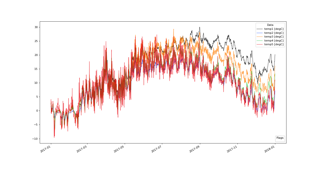
Example Algorithm Application#
Looking at the example data set more closely, we see that 2 of the 5 variables start to drift away.
2 variables are departed from the majority group of variables (the group containing more than frac variables) by the end of the year.#
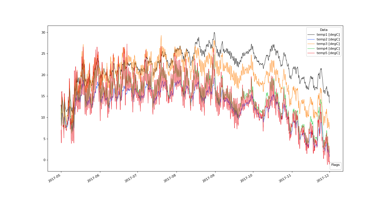
Lets try to detect those drifts via saqc. The changes we observe in the data seem to develop significantly only in temporal spans over a month,
so we go for "1ME" as value for the
window parameter. We identified the majority group as a group containing three variables, whereby two variables
seem to be scattered away, so that we can leave the frac value at its default .5 level.
The majority group seems on average not to be spread out more than 3 or 4 degrees. So, for the spread value
we go for 3. This can be interpreted as follows, for every member of a group, there is another member that
is not distanted more than 3 degrees from that one (on average in one month) - this should be sufficient to bundle
the majority group and to discriminate against the drifting variables, that seem to deviate more than 3 degrees on
average in a month from any member of the majority group.
>>> variables = ['temp1 [degC]', 'temp2 [degC]', 'temp3 [degC]', 'temp4 [degC]', 'temp5 [degC]']
>>> qc = qc.flagDriftFromNorm(variables, window='1ME', spread=3)
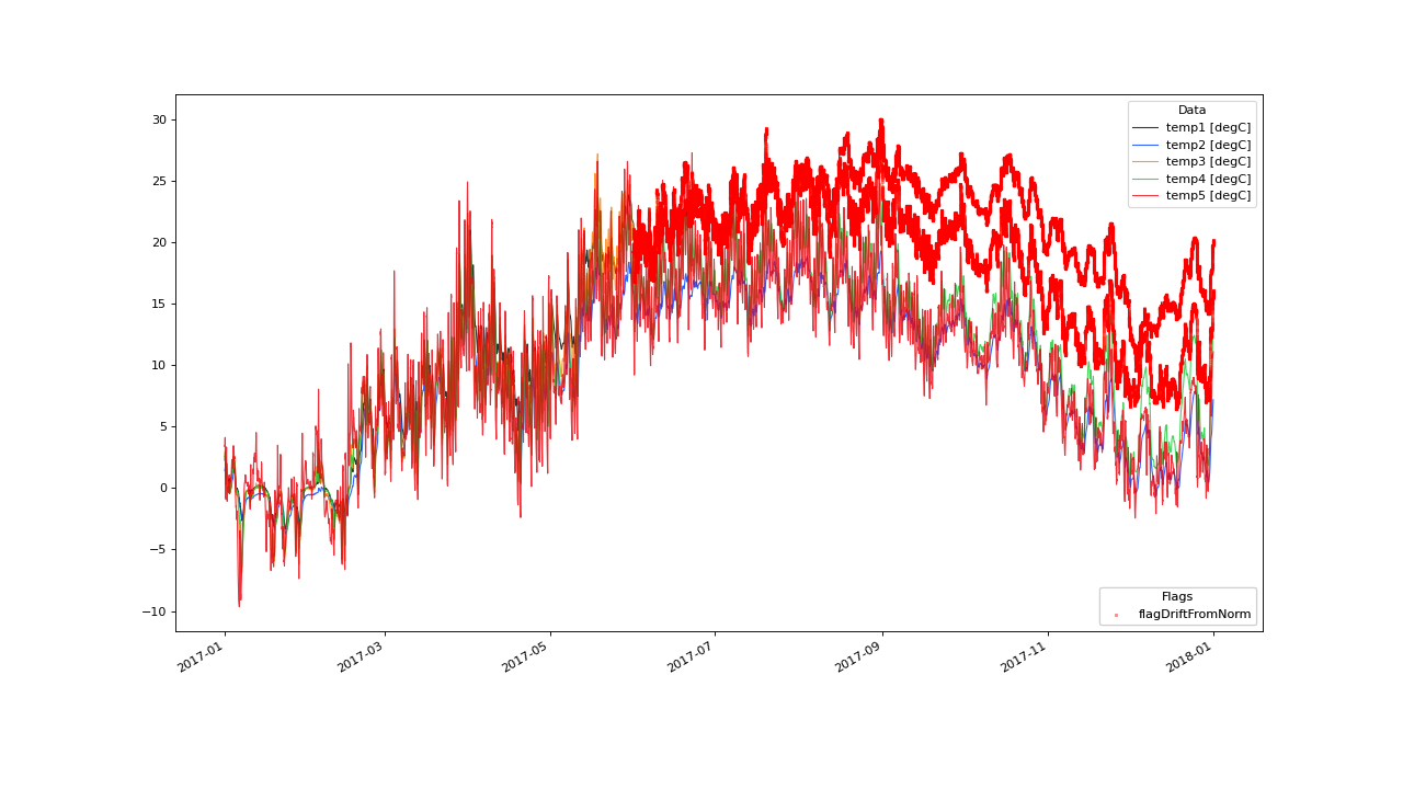
Lets check the results:
>>> qc.plot(variables, marker_kwargs={'alpha':.3, 's': 1, 'color': 'red', 'edgecolor': 'face'})