


Obtaining Residual Data and Scores for Outlier Detection#
The tutorial aims to introduce the usage of saqc methods in order to detect outliers in an uni-variate set up.
The tutorial guides through the following steps:
We checkout and load the example data set. Subsequently, we initialise an
SaQCobject.We will see how to apply different smoothing methods and models to the data in order to obtain usefull residual variables.
We will see how we can obtain residuals and scores from the calculated model curves.
Finally, we will see how to derive flags from the scores itself and impose additional conditions, functioning as correctives.
Preparation#
Data#
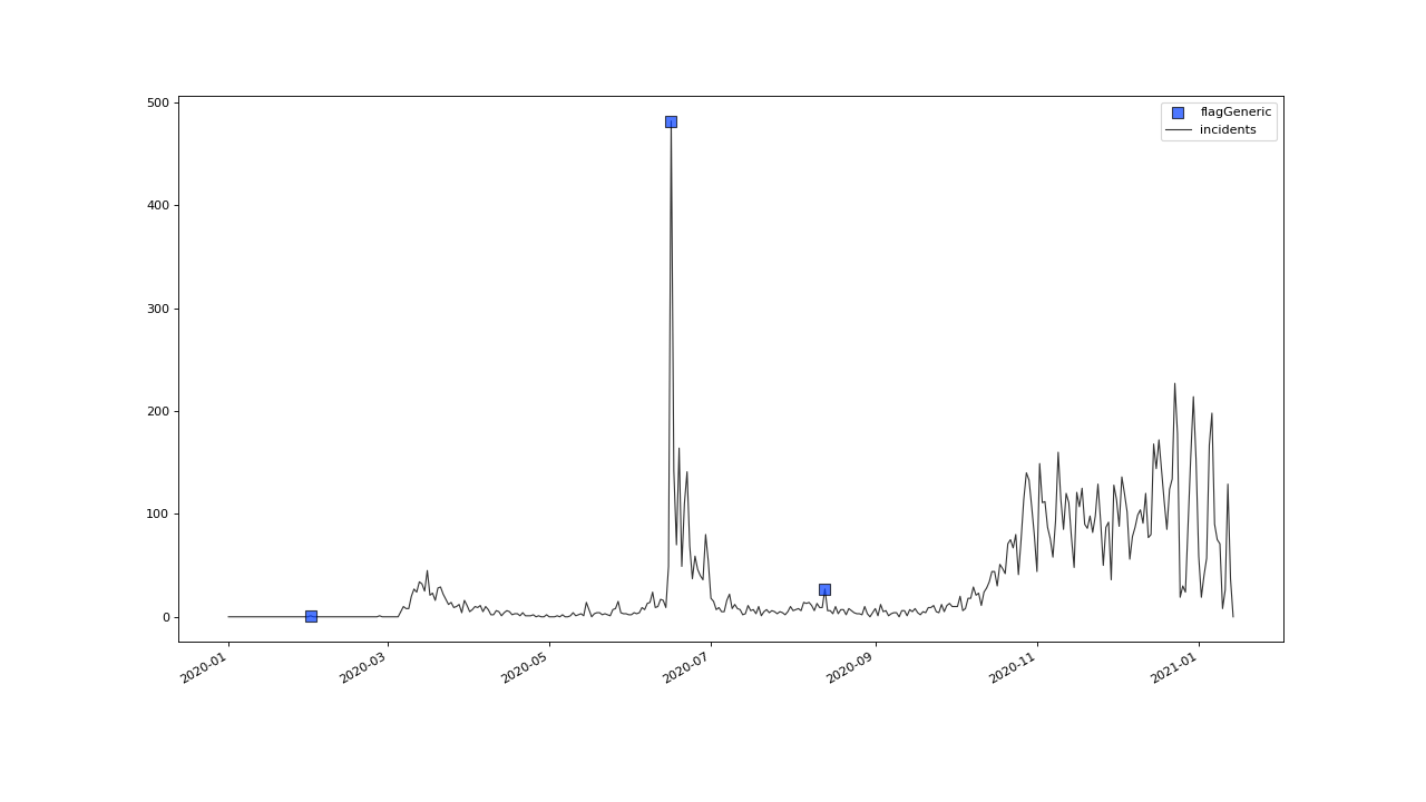
The example data set is selected to be small, comprehendable and its single anomalous outlier can be identified easily visually:
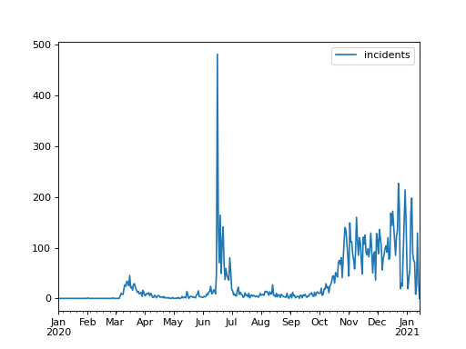
It can be downloaded from the saqc git repository.
The data represents incidents of SARS-CoV-2 infections, on a daily basis, as reported by the RKI in 2020.
In June, an extreme spike can be observed. This spike relates to an incidence of so called “superspreading” in a local meat factory.
For the sake of modelling the spread of Covid, it can be of advantage, to filter the data for such extreme events, since they may not be consistent with underlying distributional assumptions and thus interfere with the parameter learning process of the modelling. Also it can help to learn about the conditions severely facilitating infection rates.
To introduce into some basic saqc workflows, we will concentrate on classic variance based outlier detection approaches.
Initialisation#
We initially want to import the data into our workspace. Therefore we import the pandas library and use its csv file parser pd.read_csv.
>>> data_path = './resources/data/incidentsLKG.csv'
>>> import pandas as pd
>>> data = pd.read_csv(data_path, index_col=0)
The resulting data variable is a pandas data frame
object. We can generate an SaQC object directly from that. Beforehand we have to make sure, the index
of data is of the right type.
>>> data.index = pd.DatetimeIndex(data.index)
Now we do load the saqc package into the workspace and generate an instance of SaQC object,
that refers to the loaded data.
>>> import saqc
>>> qc = saqc.SaQC(data)
The only timeseries have here, is the incidents dataset. We can have a look at the data and obtain the above plot through
the method plot():
>>> qc.plot('incidents')
Modelling#
First, we want to model our data in order to obtain a stationary, residuish variable with zero mean.
Rolling Mean#
Easiest thing to do, would be, to apply some rolling mean
model via the method saqc.SaQC.rolling().
>>> import numpy as np
>>> qc = qc.rolling(field='incidents', target='incidents_mean', func=np.mean, window='13D')
The field parameter is passed the variable name, we want to calculate the rolling mean of.
The target parameter holds the name, we want to store the results of the calculation to.
The window parameter controlls the size of the rolling window. It can be fed any so called date alias string. We chose the rolling window to have a 13 days span.
Rolling Median#
You can pass arbitrary function objects to the func parameter, to be applied to calculate every single windows “score”.
For example, you could go for the median instead of the mean. The numpy library provides a median function
under the name np.median. We just calculate another model curve for the "incidents" data with the np.median function from the numpy library.
>>> qc = qc.rolling(field='incidents', target='incidents_median', func=np.median, window='13D')
We chose another target value for the rolling median calculation, in order to not override our results from
the previous rolling mean calculation.
The target parameter can be passed to any call of a function from the
saqc functions pool and will determine the result of the function to be written to the
data, under the fieldname specified by it. If there already exists a field with the name passed to target,
the data stored to this field will be overridden.
We will evaluate and visualize the different model curves later. Beforehand, we will generate some more model data.
Polynomial Fit#
Another common approach, is, to fit polynomials of certain degrees to the data.
SaQC provides the polynomial fit function fitPolynomial():
>>> qc = qc.fitPolynomial(field='incidents', target='incidents_polynomial', order=2, window='13D')
It also takes a window parameter, determining the size of the fitting window.
The parameter, order refers to the size of the rolling window, the polynomials get fitted to.
Custom Models#
If you want to apply a completely arbitrary function to your data, without pre-chunking it by a rolling window,
you can make use of the more general processGeneric() function.
Lets apply a smoothing filter from the scipy.signal module. We wrap the filter generator up into a function first:
from scipy.signal import filtfilt, butter
def butterFilter(x, filter_order, nyq, cutoff, filter_type="lowpass"):
    b, a = butter(N=filter_order, Wn=cutoff / nyq, btype=filter_type)
    return pd.Series(filtfilt(b, a, x), index=x.index)
This function object, we can pass on to the processGeneric() methods func argument.
>>> qc = qc.processGeneric(field='incidents', target='incidents_lowPass',
... func=lambda x: butterFilter(x, cutoff=0.1, nyq=0.5, filter_order=2))
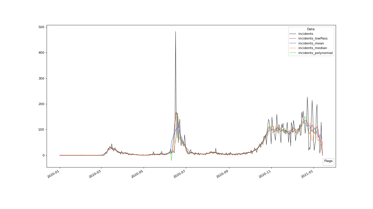
Visualisation#
To see all the results obtained so far, plotted in one figure window, we make use of the plot() method.
>>> qc.plot(".", regex=True)
Residuals and Scores#
Residuals#
We want to evaluate the residuals of one of our models model, in order to score the outlierish-nes of every point. Therefor we just stick to the initially calculated rolling mean curve.
First, we retrieve the residuals via the processGeneric() method.
This method always comes into play, when we want to obtain variables, resulting from basic algebraic
manipulations of one or more input variables.
For obtaining the models residuals, we just subtract the model data from the original data and assign the result
of this operation to a new variable, called incidents_residuals. This Assignment, we, as usual,
control via the target parameter.
>>> qc = qc.processGeneric(['incidents', 'incidents_mean'], target='incidents_residuals', func=lambda x, y: x - y)
Scores#
Next, we score the residuals simply by computing their Z-scores. The Z-score of a point \(x\), relative to its surrounding \(D\), evaluates to \(Z(x) = \frac{x - \mu(D)}{\sigma(D)}\).
So, if we would like to roll with a window of a fixed size of 27 periods through the data and calculate the Z-score
for the point lying in the center of every window, we would define our function z_score:
>>> z_score = lambda D: abs((D[14] - np.mean(D)) / np.std(D))
And subsequently, use the rolling() method to make a rolling window application with the scoring
function:
>>> qc = qc.rolling(field='incidents_residuals', target='incidents_scores', func=z_score, window='27D', min_periods=27)
Optimization by Decomposition#
There are 2 problems with the attempt presented above.
First, the rolling application of the customly
defined function, might get really slow for large data sets, because our function z_scores does not get decomposed into optimized building blocks.
Second, and maybe more important, it relies heavily on every window having a fixed number of values and a fixed temporal extension.
Otherwise, D[14] might not always be the value in the middle of the window, or it might not even exist,
and an error will be thrown.
So the attempt works fine, only because our data set is small and strictly regularily sampled. Meaning that it has constant temporal distances between subsequent meassurements.
In order to tweak our calculations and make them much more stable, it might be useful to decompose the scoring
into seperate calls to the rolling() function, by calculating the series of the
residuals mean and standard deviation seperately:
>>> qc = qc.rolling(field='incidents_residuals', target='residuals_mean', window='27D', func=np.mean)
>>> qc = qc.rolling(field='incidents_residuals', target='residuals_std', window='27D', func=np.std)
>>> qc = qc.processGeneric(field=['incidents_scores', "residuals_mean", "residuals_std"], target="residuals_norm",
... func=lambda this, mean, std: (this - mean) / std)
With huge datasets, this will be noticably faster, compared to the method presented initially,
because saqc dispatches the rolling with the basic numpy statistic methods to an optimized pandas built-in.
Also, as a result of the rolling() assigning its results to the center of every window,
all the values are centered and we dont have to care about window center indices when we are generating
the Z-Scores from the two series.
We simply combine them via the
processGeneric() method, in order to obtain the scores:
>>> qc = qc.processGeneric(field=['incidents_residuals','residuals_mean','residuals_std'],
... target='incidents_scores', func=lambda x,y,z: abs((x-y) / z))
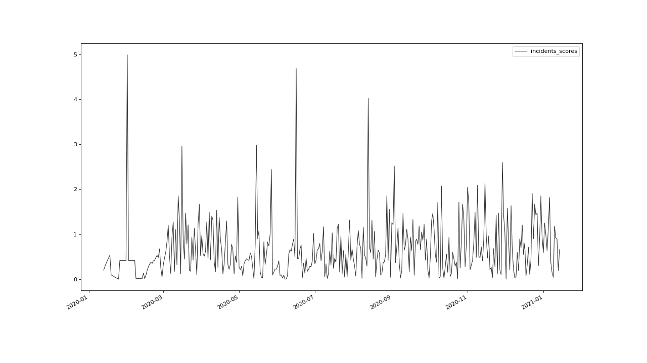
Let’s have a look at the resulting scores:
>>> qc.plot('incidents_scores')
Setting and correcting Flags#
Flagging the Scores#
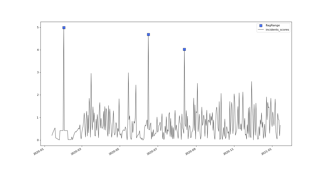
We can now implement the common rule of thumb,
that any Z-score value above 3 may indicate an outlierish data point,
by applying the flagRange() method with a max value of 3.
>>> qc = qc.flagRange('incidents_scores', max=3)
Now flags have been calculated for the scores:
>>> qc.plot('incidents_scores')
Projecting Flags#
We now can project those flags onto our original incidents timeseries:
>>> qc = qc.flagGeneric(field=['incidents_scores'], target='incidents', func=lambda x: isflagged(x))
Note, that we could have skipped the range flagging step, by including the cutting off in our
generic expression:
>>> qc = qc.flagGeneric(field=['incidents_scores'], target='incidents', func=lambda x: x > 3)
Lets check out the results:
>>> qc.plot('incidents')
Obveously, there are some flags set, that, relative to their 13 days surrounding, might relate to minor incidents spikes, but may not relate to superspreading events we are looking for.
Especially the left most flag seems not to relate to an extreme event at all. This overflagging stems from those values having a surrounding with very low data variance, and thus, evaluate to a relatively high Z-score.
There are a lot of possibilities to tackle the issue. In the next section, we will see how we can improve the flagging results by incorporating additional domain knowledge.
Additional Conditions#
In order to improve our flagging result, we could additionally assume, that the events we are interested in, are those with an incidents count that is deviating by a margin of more than 20 from the 2 week average.
This is equivalent to imposing the additional condition, that an outlier must relate to a sufficiently large residual.
Unflagging#
We can do that posterior to the preceeding flagging step, by removing some flags based on some condition.
In order want to unflag those values, that do not relate to
sufficiently large residuals, we assign them the UNFLAGGED flag.
Therefore, we make use of the flagGeneric() method.
This method usually comes into play, when we want to assign flags based on the evaluation of logical expressions.
So, we check out, which residuals evaluate to a level below 20, and assign the
flag value for UNFLAGGED. This value defaults to
to -np.inf in the default translation scheme, wich we selected implicitly by not specifying any special scheme in the
generation of the SaQC> object in the beginning.
>>> qc = qc.flagGeneric(field=['incidents','incidents_residuals'], target="incidents",
... func=lambda x,y: isflagged(x) & (y < 50), flag=-np.inf)
Notice, that we passed the desired flag level to the flag keyword in order to perform an
“unflagging” instead of the usual flagging. The flag keyword can be passed to all the functions
and defaults to the selected translation schemes BAD flag level.
Plotting proofs the tweaking did in deed improve the flagging result:
>>> qc.plot("incidents")

Including multiple conditions#
If we do not want to first set flags, only to remove the majority of them in the next step, we also
could circumvent the unflagging step, by adding to the call to
flagRange() the condition for the residuals having to be above 20
>>> qc = qc.flagGeneric(field=['incidents_scores', 'incidents_residuals'], target='incidents',
... func=lambda x, y: (x > 3) & (y > 20))
>>> qc.plot("incidents")
